Process management

Introduction to Process management

Process management is a crucial aspect of operating systems (OS) that deals with the creation, scheduling, and termination of processes. Here’s an overview:

What is a Process?

A process is an instance of a program in execution. It comprises the program code, its current activity, and the resources it uses (like CPU time, memory, and I/O devices). Each process operates independently and can be in various states (e.g., running, waiting, or terminated).

Key Concepts in Process Management

1. Process Creation:
   • Fork: A process can create a new process using a system call like fork (in Unix-like systems). The new process, known as the child process, is a duplicate of the parent process.
   • Exec: After creation, a process can replace its memory space with a new program using system calls like exec. This is often done to run different programs.
2. Process Scheduling:
   • Scheduling: The OS must decide which process runs at any given time. This involves algorithms like Round-Robin, First-Come-First-Serve, and Priority Scheduling.
   • Context Switching: When switching between processes, the OS saves the state of the current process and loads the state of the next process. This operation is called context switching.
3. Process States:
   • New: The process is being created.
   • Ready: The process is waiting to be assigned to a processor.
   • Running: The process is currently being executed by the CPU.
   • Waiting: The process is waiting for some event (e.g., I/O completion).
   • Terminated: The process has finished execution.
4. Process Control Block (PCB):
   • The PCB is a data structure used by the OS to manage process information. It contains details like the process state, program counter, CPU registers, memory management information, and process ID.
5. Inter-Process Communication (IPC):
   • IPC mechanisms allow processes to communicate and synchronize with each other. Common methods include pipes, message queues, and shared memory.
6. Synchronization and Deadlock:
   • Synchronization: Ensures that processes or threads do not interfere with each other when accessing shared resources.
   • Deadlock: A situation where processes are unable to proceed because each is waiting for resources held by the others. The OS must implement strategies to prevent, avoid, or recover from deadlock.

Advantages of Efficient Process Management

1. Optimized CPU Utilization: Efficient scheduling and management lead to better CPU usage.
2. Improved System Throughput: Proper management can increase the number of processes completed in a given time.
3. Enhanced User Experience: Ensures smooth and responsive system performance by effectively handling multiple tasks.

Disadvantages of Process Management Complexity

1. Overhead: Managing processes requires system resources and can add overhead, especially with frequent context switching.
2. Deadlock Issues: Complex scenarios can lead to deadlocks if not managed correctly.
3. Resource Contention: Processes may compete for limited resources, potentially affecting performance.

Overall, effective process management ensures that the system runs smoothly, balancing the needs of various processes and optimizing the use of system resources.

Difference between Process and Program

Aspect	Program	Process
Definition	A set of instructions written to perform a task	An instance of a program in execution
State	Static (does not change state)	Dynamic (can be in various states: New, Ready, Running, Waiting, Terminated)
Existence	Exists as a file on disk	Exists in the memory and is being executed
Resource Usage	Does not use system resources actively	Actively uses CPU, memory, and other system resources
Creation	Created when written and saved to storage	Created when a program is executed
Lifecycle	Lifelong as a file until deleted	Lifecycle includes creation, execution, and termination
Execution	Not executable by itself	Executes instructions and performs tasks
Memory	Resides in secondary storage (e.g., hard drive)	Resides in primary memory (RAM) while running
Interaction	Does not interact with other programs or processes	Can interact with other processes through IPC
Example	example_program.exe	An instance of example_program.exe running

In summary, a program is a static set of instructions stored on disk, while a process is a dynamic entity that represents the execution of a program, actively using system resources and undergoing various state transitions.

Define process

A process is an instance of a program in execution. It includes the program code, its current activity, and the resources it uses (such as CPU time, memory, and I/O devices). A process is a fundamental unit of work in a computer system, managed by the operating system.

Key Components of a Process

1. Program Code: The executable instructions that make up the program.
2. Program Counter: A register that holds the address of the next instruction to be executed.
3. Process Stack: Contains temporary data such as function parameters, return addresses, and local variables.
4. Process Heap: Used for dynamic memory allocation during the process’s execution.
5. Process State: Indicates the current status of the process (e.g., new, ready, running, waiting, terminated).
6. Process Control Block (PCB): A data structure used by the OS to store information about the process, including its state, program counter, CPU registers, memory management information, and process ID.

Process States

1. New: The process is being created.
2. Ready: The process is waiting to be assigned to a CPU.
3. Running: The process is currently being executed by the CPU.
4. Waiting: The process is waiting for some event (e.g., I/O completion).
5. Terminated: The process has finished execution.

Characteristics

• Execution: A process can execute instructions and perform tasks while in the running state.
• Isolation: Processes operate independently and are isolated from each other, although they can communicate through Inter-Process Communication (IPC) mechanisms.
• Resource Usage: Each process uses system resources such as CPU time, memory, and I/O devices, and the OS manages these resources to ensure efficient execution and prevent conflicts.

In essence, a process represents a program in action, encompassing everything needed for the program to run and interact with the system.

Sequential Process

A sequential process is one that executes its instructions in a linear, step-by-step manner without any concurrent or parallel execution. This means each instruction is executed one after the other, and the process proceeds from one step to the next in a predetermined order.

Characteristics of Sequential Processes

1. Linear Execution: Instructions are executed in a strict sequence, one after the other.
2. Single Thread: Typically involves a single thread of execution, meaning only one operation is performed at any given time.
3. Predictable Behavior: Since there is no parallelism or concurrency, the behavior of the process is predictable and straightforward.
4. Simple to Implement: Sequential processes are easier to design and debug because of their straightforward execution flow.

Advantages

1. Simplicity: Easier to understand and implement due to the linear flow of control.
2. Consistency: Avoids issues related to concurrent execution, such as race conditions and synchronization problems.
3. Predictability: Execution order is predictable, making it easier to trace and debug.

Disadvantages

1. Limited Performance: Sequential processes can be less efficient compared to concurrent or parallel processes, especially for tasks that could benefit from simultaneous execution.
2. Scalability Issues: Sequential execution does not take advantage of multi-core processors or distributed systems, potentially leading to performance bottlenecks in more complex or resource-intensive applications.

Examples

• Basic Calculator: Performing arithmetic operations one after another without needing to manage multiple tasks concurrently.
• Simple Data Processing: Reading data from a file, processing it, and then writing the results back to a file in a single, continuous flow.

In summary, a sequential process is characterized by its step-by-step execution where each operation follows the previous one in a single thread of control, making it simple but potentially less efficient for complex tasks requiring parallelism.

Sequential Process Example: File Processing

Steps Involved:

1. Open Input File: The process starts by opening the file that contains the data.
2. Read Data: The process reads the data from the input file.
3. Process Data: The process performs operations on the data (e.g., computations or transformations).
4. Write Output: The process writes the processed data to an output file.
5. Close Files: The process closes both the input and output files.

Diagram

Here’s a diagram illustrating the sequential flow of this process:

+-----------------+      +------------------+      +------------------+
| Open Input File | ---> | Read Data        | ---> | Process Data     |
+-----------------+      +------------------+      +------------------+
                                                           |
                                                           v
                                                +------------------+
                                                | Write Output     |
                                                +------------------+
                                                           |
                                                           v
                                                +------------------+
                                                | Close Files      |
                                                +------------------+

Explanation

1. Open Input File: The process starts by opening the file for reading.
2. Read Data: The data is read from the file in a sequential manner.
3. Process Data: The data is then processed step-by-step.
4. Write Output: After processing, the result is written to an output file.
5. Close Files: Finally, both files are closed to release system resources.

In this sequential process, each step must be completed before the next one begins. There is no overlap or parallel execution; each task is performed in a strict order. This simplicity ensures that the process is easy to follow but may not be the most efficient for tasks that could benefit from concurrent or parallel execution.

Process control block

A Process Control Block (PCB) is a data structure used by the operating system to manage information about a process. It is crucial for process management and keeps track of the various attributes of a process. Here’s a breakdown of what a PCB typically contains:

Components of a PCB

1. Process ID (PID): A unique identifier assigned to each process.
2. Process State: The current state of the process (e.g., running, waiting, ready).
3. Program Counter (PC): The address of the next instruction to be executed for the process.
4. CPU Registers: The values of the CPU registers when the process was last running, so they can be restored when the process resumes.
5. Memory Management Information: Details such as the base and limit registers, page tables, or segment tables, depending on the memory management scheme used.
6. Scheduling Information: Data related to process scheduling, such as priority, scheduling queues, and time slices.
7. I/O Status Information: Information about the I/O devices allocated to the process and their status.
8. Accounting Information: Statistics and information related to resource usage, such as CPU time used and execution time.

Functions of a PCB

1. Process Scheduling: The PCB allows the operating system to manage processes efficiently by storing necessary information for scheduling and context switching.
2. Context Switching: During context switching, the state of the CPU is saved into the PCB of the currently running process and restored from the PCB of the process being scheduled to run.
3. Process Management: It helps in managing the process’s execution, memory, and resources, and allows for process creation and termination.

Advantages of Using PCBs

• Efficient Process Management: Provides a structured way to keep track of multiple processes.
• Context Switching: Facilitates the smooth transition of process states and CPU context, allowing multitasking.
• Resource Tracking: Helps in tracking resources used by processes, enabling better resource allocation and management.

Disadvantages of Using PCBs

• Overhead: Maintaining and updating PCBs requires memory and processing time.
• Complexity: Managing and maintaining a large number of PCBs can add complexity to the operating system.

In summary, the PCB is essential for the smooth operation of an operating system, enabling efficient process management and multitasking.

process state diagram

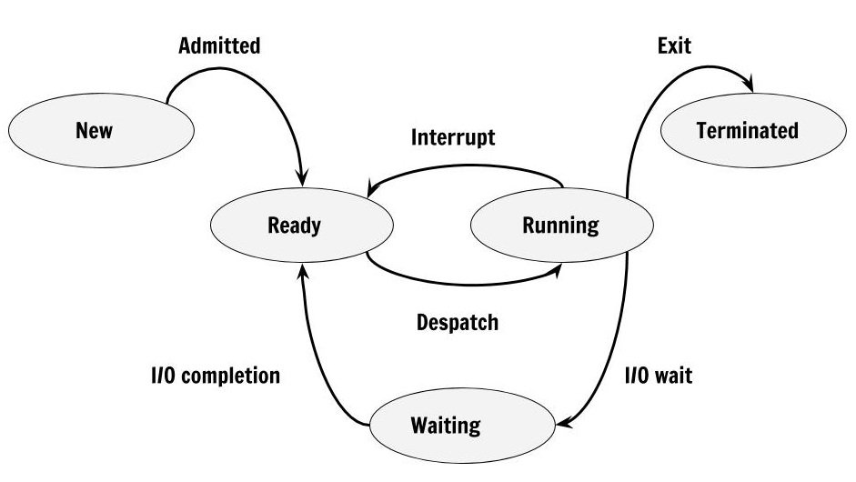
In an operating system, a process is a program that’s currently being executed. As it runs, it can be in various states. Knowing these states helps us understand how the operating system manages processes and keeps the computer running smoothly.

Here are the main process states:

1. New State: The process is being created but isn’t fully created yet. It’s just a program in secondary memory that the OS will use to make the process.
2. Ready State: Once the process is created, it moves to the ready state. Here, the process is loaded into main memory and is waiting for CPU time to start running. Processes in this state are kept in a “ready queue.”
3. Run State: The process is selected from the ready queue by the OS and is now running. The CPU executes the instructions of the process.
4. Blocked or Wait State: If the process needs something, like user input or access to an I/O device, it moves to the blocked state. It waits in main memory but doesn’t use the CPU. Once the needed resource becomes available, the process goes back to the ready state.
5. Terminated or Completed State: The process finishes its execution or is terminated. The OS removes it, frees up any resources it was using, and deletes its process control block (PCB).

Additionally, there are two more states related to memory management:

• Suspend Ready: A process that was ready but swapped out of main memory to external storage (like a hard drive) is in this state. It will return to the ready state when it’s brought back into main memory.
• Suspend Wait or Suspend Blocked: A process that was waiting for an I/O operation and was swapped out of memory is in this state. It will move to the suspend ready state when the I/O operation finishes.

CPU and I/O Bound Processes

• CPU Bound Process: This process needs a lot of CPU time to complete.
• I/O Bound Process: This process needs a lot of input/output operations to complete.

How a Process Moves Between States

1. New to Ready: When a process is created and has its resources allocated, it moves to the ready state.
2. Ready to Running: When the CPU is free, the OS selects a process from the ready queue to run.
3. Running to Blocked: If the process needs to wait for something (like user input), it moves to the blocked state.
4. Running to Ready: If a higher-priority process needs CPU time, the current process may be moved back to the ready state.
5. Blocked to Ready: When the event the process was waiting for happens, it moves back to the ready state.
6. Running to Terminated: When the process finishes or is killed, it moves to the terminated state.

Process Creation and Termination

In an operating system, processes are fundamental units of execution. Understanding how processes are created and terminated is crucial for grasping how an OS manages tasks.

Process Creation

The process creation involves several steps:

1. Process Initialization:
   • When a new process needs to be started, the operating system allocates memory for the process, sets up the necessary data structures (like the Process Control Block, or PCB), and initializes the process’s state.
2. Loading:
   • The program code, along with any initial data, is loaded into the process’s allocated memory space. This is typically done from secondary storage (like a hard drive) into the main memory.
3. Setting Up Execution:
   • The OS sets up the process’s execution context, which includes the CPU registers, program counter, and stack. This prepares the process to be executed by the CPU.
4. Process Scheduling:
   • The new process is then placed in the ready queue, waiting for CPU time. The operating system’s scheduler will eventually select it to run based on its scheduling algorithm.
5. Starting Execution:
   • Once scheduled, the process transitions from the ready state to the running state and begins execution.

Example: When you start a new application on your computer, the OS creates a new process for it, allocating memory and setting up the necessary resources before running it.

Process Termination

A process may terminate for various reasons. The termination process includes:

1. Normal Completion:
   • The process completes its execution by running to the end of its code. It will then exit gracefully, often signaling completion to the operating system.
2. Error or Exception:
   • The process may encounter an error or exception that prevents it from continuing. In this case, it may terminate abnormally, and the OS will handle the error and clean up resources.
3. Forced Termination:
   • Sometimes, the operating system or a user may forcefully terminate a process. This might be necessary if the process is misbehaving or consuming excessive resources.
4. Resource Deallocation:
   • Upon termination, the OS releases any resources allocated to the process, including memory, I/O devices, and any other system resources. The process control block (PCB) associated with the process is also deleted.
5. Cleanup:
   • The operating system performs any necessary cleanup operations, such as updating system tables and freeing memory. This ensures that the system remains stable and that resources are available for other processes.

Example: When you close an application, the operating system terminates the process associated with that application. It releases the memory and other resources that were being used by the application.

Summary

• Process Creation: Involves initialization, loading program code, setting up execution context, scheduling, and starting execution.
• Process Termination: Occurs through normal completion, error handling, or forced termination, followed by resource deallocation and cleanup.

This process lifecycle ensures that the operating system can efficiently manage multiple processes, allocate resources, and maintain system stability.

Relation Between Processes

In an operating system, processes can have various relationships with each other, primarily due to process creation, communication, and resource sharing. Understanding these relationships is essential for managing how processes interact and ensuring efficient system performance.

Parent and Child Processes

Parent Process

• A parent process is a process that creates one or more child processes.
• When a parent process creates a child process, it typically uses system calls like fork() in UNIX/Linux systems or CreateProcess() in Windows.

Child Process

• A child process is a process that is created by another process (the parent).
• Child processes inherit certain attributes from their parent, such as environment variables, open files, and more.
• The child process may execute the same program as the parent or a different one, depending on how it’s configured.

Example:

• In UNIX/Linux, when you run a shell command, the shell creates a child process to execute the command.

Process Hierarchy

• Process Tree:
  • In a system, processes can be arranged in a tree-like structure where each process may have multiple children. This hierarchy is known as a process tree.
  • The root of this tree is often a special process like init (or systemd in Linux), which is the ancestor of all processes.
• Process Group:
  • A process group is a collection of related processes that can be managed as a unit. For example, when you run a command in a shell pipeline, all processes involved in the pipeline are part of the same process group.
  • Process groups are used to control terminal access and signal distribution.

Inter-Process Communication (IPC)

Processes often need to communicate with each other to share data or coordinate actions. Various mechanisms are used for Inter-Process Communication:

1. Pipes:
   • Pipes are used for unidirectional data flow between two processes. A pipe allows one process to send data to another.
2. Message Queues:
   • Message queues provide a way for processes to exchange messages in a structured way. This allows for asynchronous communication between processes.
3. Shared Memory:
   • Shared memory allows multiple processes to access the same memory space, facilitating fast data exchange. It requires synchronization mechanisms to manage access.
4. Semaphores:
   • Semaphores are used to synchronize access to resources, preventing race conditions and ensuring that only one process can access a critical section at a time.
5. Sockets:
   • Sockets allow processes to communicate over a network, supporting both local and remote communication.

Process Synchronization

Processes often need to synchronize their actions to ensure correct execution. This is crucial when processes share resources or data.

• Mutexes (Mutual Exclusion):
  • Mutexes are used to ensure that only one process can access a critical section of code at any given time, preventing data corruption.
• Locks:
  • Locks are mechanisms that prevent multiple processes from accessing shared resources simultaneously.
• Barriers:
  • Barriers are synchronization points where processes must wait until all processes reach the barrier before any can proceed.

Summary

• Parent and Child Processes: Processes can create child processes, forming a hierarchical structure.
• Process Hierarchy: Processes can be organized in a tree or groups for management.
• Inter-Process Communication: Processes communicate through pipes, message queues, shared memory, semaphores, and sockets.
• Process Synchronization: Processes synchronize using mutexes, locks, and barriers to ensure data integrity.
• Orphan and Zombie Processes: Orphan processes are adopted by the init process, while zombie processes are terminated but not yet reaped by their parent.

Understanding the relationships between processes is crucial for designing efficient and robust applications that can leverage parallel execution and resource sharing.

Threads are a fundamental concept in operating systems and concurrent programming, providing a way to achieve parallelism within a single process. They enable efficient use of system resources and improve the responsiveness and performance of applications. Let’s explore what threads are and how they work.

What are Threads?

• Definition: A thread is the smallest unit of execution within a process. It represents a single sequence of instructions that can be executed independently by a CPU.

Real-Life Example: Restaurant Kitchen

Imagine a restaurant kitchen where multiple chefs work simultaneously to prepare a meal. Each chef is like a thread, performing specific tasks such as chopping vegetables, grilling meat, or plating dishes. These chefs work concurrently, sharing resources such as kitchen utensils and the stove. Let’s break down this analogy to understand threads better:

Components of a Threaded System in a Restaurant

1. Chefs (Threads):
   • Tasks: Each chef performs a specific task, much like how each thread executes a particular portion of code.
   • Concurrency: Chefs work at the same time, allowing the meal to be prepared faster. Similarly, threads run concurrently, improving application performance.
2. Kitchen (Process):
   • Shared Resources: All chefs share resources like ingredients, cooking tools, and workspace, just as threads share memory and other resources within a process.
   • Coordination: Chefs must coordinate to avoid conflicts, such as using the same pan simultaneously. Threads must also synchronize to prevent data corruption and ensure consistent results.
3. Meal Preparation (Task Completion):
   • Efficiency: By dividing tasks among chefs, the meal is prepared more efficiently. Threads allow an application to break tasks into smaller parts, executing them concurrently for faster completion.
4. Synchronization:
   • Timing: Chefs must time their tasks so that dishes are ready simultaneously. In software, threads use synchronization mechanisms like locks and semaphores to coordinate execution.
5. Challenges:
   • Conflicts: If two chefs try to use the same ingredient simultaneously, conflicts may arise. Threads can experience race conditions when accessing shared data, requiring careful synchronization.
   • Overhead: More chefs in the kitchen can lead to overcrowding and inefficiencies. Similarly, too many threads can cause resource contention and increased context-switching overhead.

Characteristics of Threads

• Shared Resources:
  • Threads within the same process share the same memory space, including the code, data, and heap segments.
  • This sharing allows threads to communicate with each other more easily and efficiently compared to separate processes, which require inter-process communication mechanisms.
• Independent Execution:
  • Each thread has its own stack, registers, and program counter, enabling it to execute independently of other threads.
  • Threads can be scheduled by the operating system to run on different CPU cores, allowing for true parallelism in multi-core systems.
• Lightweight:
  • Creating and managing threads is generally more efficient and less resource-intensive than creating and managing full processes.
  • This is because threads share resources, such as memory and files, which reduces the overhead associated with context switching between threads compared to processes.

Advantages of Using Threads

1. Improved Performance:
   • Threads can run concurrently, improving the responsiveness and throughput of applications.
   • Applications that perform tasks like handling multiple client requests or processing large datasets can benefit significantly from multithreading.
2. Responsiveness:
   • In graphical user interfaces (GUIs), threads can keep the interface responsive while performing background tasks.
   • For example, a text editor can continue to accept user input while saving a document in the background.
3. Resource Sharing:
   • Threads within the same process can easily share data and resources, simplifying the development of concurrent applications.
4. Scalability:
   • Multithreaded applications can take advantage of multi-core processors, distributing tasks across multiple cores to achieve better scalability and performance.

Disadvantages of Using Threads

1. Complexity:
   • Writing multithreaded applications can be complex and error-prone, requiring careful synchronization to avoid race conditions and deadlocks.
   • Developers must ensure proper use of synchronization primitives, such as mutexes and semaphores, to manage access to shared resources.
2. Debugging Challenges:
   • Debugging multithreaded applications can be challenging due to non-deterministic execution, making it difficult to reproduce and diagnose issues.
3. Overhead:
   • While threads are lighter than processes, they still introduce some overhead in terms of context switching and synchronization.

Use Cases for Threads

Threads are widely used in various applications and systems:

• Web Servers: Handle multiple client requests simultaneously by assigning each request to a separate thread.
• Graphical User Interfaces: Keep the UI responsive by performing long-running tasks in background threads.
• Data Processing: Divide large datasets into smaller chunks and process them in parallel using threads.
• Real-Time Systems: Achieve concurrency in real-time systems where tasks must be executed simultaneously to meet deadlines.

Conclusion

Threads are essential for modern computing, enabling applications to perform multiple tasks concurrently and efficiently. By leveraging threads, developers can create responsive, high-performance applications that take full advantage of multi-core processors. However, writing multithreaded applications requires careful consideration of synchronization and resource management to avoid common pitfalls like race conditions and deadlocks.

Differences Between Processes and Threads

Aspect	Process	Thread
Memory	Each process has its own memory space (address space).	Threads share the same memory space within a process.
Communication	Inter-process communication (IPC) is required, which can be slower and more complex.	Threads can communicate more easily by sharing data directly in the same memory space.
Isolation	Processes are isolated from each other, providing protection against crashes.	Threads are not isolated, so a crash in one thread can affect the entire process.
Creation	Creating a process is relatively heavy and slow.	Threads are lightweight, and creating them is faster and less resource-intensive.
Context Switching	Context switching between processes is more expensive due to different memory spaces.	Context switching between threads is cheaper since they share the same memory space.
Resource Allocation	Processes have separate resources like file handles, memory, etc.	Threads share resources such as file handles, memory, and data within the process.
Execution	Processes run independently; each process has its own execution environment.	Threads run concurrently within the same process, sharing the same execution environment.
Security	Processes offer better security and stability since they do not share memory.	Threads can potentially lead to data inconsistency and require careful synchronization.

Multithreading is a powerful programming concept that allows multiple threads to be executed concurrently within a single process. This can significantly improve the performance and responsiveness of applications, especially in multi-core processor environments. Let’s explore multithreading in detail, including its benefits, challenges, and real-world applications.

What is Multithreading?

• Definition: Multithreading is the ability of a CPU, or a single core within a multi-core processor, to execute multiple threads simultaneously. It allows a process to perform multiple tasks concurrently, utilizing CPU resources more efficiently.
• Concurrency vs. Parallelism:
  • Concurrency: Refers to multiple threads making progress at the same time. This can be achieved on a single-core processor by context switching between threads.
  • Parallelism: Refers to multiple threads running simultaneously on different cores of a multi-core processor, allowing true parallel execution.

Real-Life Example: A Restaurant Kitchen

Imagine a busy restaurant kitchen where multiple chefs are working simultaneously to prepare a variety of dishes. Each chef focuses on different tasks, such as chopping vegetables, cooking meat, or baking desserts. This scenario is analogous to a multithreaded application where each thread handles a specific task. Let’s break down this analogy:

Components of a Multithreaded Kitchen

1. Chefs as Threads:
   • Specialized Tasks: Each chef (thread) has a specific role, such as grilling, baking, or making salads. Similarly, in a multithreaded application, each thread performs a specific task, like handling user input, processing data, or rendering graphics.
   • Concurrent Execution: Chefs work simultaneously, just as threads run concurrently. This concurrency allows the kitchen (application) to serve more customers efficiently by preparing multiple dishes at once.
2. Kitchen as a Process:
   • Shared Resources: All chefs share kitchen resources like ovens, stoves, utensils, and ingredients, much like threads share memory and resources within a process.
   • Coordination: Chefs must coordinate to avoid conflicts, such as using the same oven simultaneously. Threads also need synchronization to prevent data corruption when accessing shared resources.
3. Order Handling:
   • Efficient Workflow: Orders (tasks) are divided among chefs, enabling the kitchen to prepare multiple orders quickly. In software, multithreading allows tasks to be divided among threads, improving performance and responsiveness.
   • Parallel Execution: Dishes that require different cooking methods can be prepared in parallel. Similarly, threads can execute tasks concurrently on multiple CPU cores, leveraging parallel processing capabilities.
4. Challenges:
   • Race Conditions: If two chefs try to use the same ingredient or equipment simultaneously, conflicts may arise. In software, race conditions occur when multiple threads access shared data without proper synchronization, leading to inconsistent results.
   • Deadlocks: If one chef waits indefinitely for another to finish using a critical resource, the kitchen could come to a standstill. Threads can experience deadlocks when they wait for each other to release resources, halting progress.

Benefits of Multithreading

1. Improved Performance:
   • By executing multiple threads concurrently, applications can utilize CPU resources more effectively, leading to faster execution times.
   • Multithreading allows applications to take advantage of multi-core processors, distributing tasks across cores for parallel execution.
2. Responsiveness:
   • Multithreading can keep applications responsive by performing background tasks while the main thread handles user interactions.
   • For example, a graphical user interface (GUI) application can remain responsive to user input while performing tasks like file I/O or network communication in separate threads.
3. Resource Sharing:
   • Threads within the same process share memory and resources, allowing for efficient communication and data exchange between threads.

Real-World Applications of Multithreading

1. Web Servers:
   • Web servers handle multiple client requests simultaneously by assigning each request to a separate thread.
   • Threads enable web servers to process multiple requests concurrently, improving throughput and responsiveness.
2. Multimedia Applications:
   • Video players and audio editors use threads to decode media, process effects, and update the user interface concurrently.
   • Multithreading allows multimedia applications to perform tasks like video rendering, audio playback, and user input processing simultaneously.
3. Games:
   • Games use threads for rendering graphics, handling physics calculations, processing AI logic, and managing user input.
   • Multithreading enables games to leverage multi-core processors, improving performance and delivering a smoother gaming experience.

Conclusion

Multithreading is a powerful tool for improving application performance and responsiveness by enabling concurrent task execution. In a restaurant kitchen, multiple chefs work together to prepare meals efficiently, just as threads in a multithreaded application perform tasks concurrently. By understanding the benefits and challenges of multithreading, developers can design applications that leverage parallelism to achieve better performance, scalability, and user experience. Whether it’s a busy kitchen or a high-performance web server, multithreading plays a crucial role in achieving efficient and responsive execution.

Scheduling Concepts

Scheduling in computer systems is a critical concept that deals with the order and allocation of system resources to various tasks. The goal is to improve system performance, responsiveness, and resource utilization. Here are some key scheduling concepts, along with explanations of different scheduling algorithms and their advantages and disadvantages:

Types of Scheduling

1. CPU Scheduling
   • Definition: Decides which process in the ready queue should be assigned to the CPU.
   • Goal: Maximize CPU utilization, throughput, and response time while minimizing waiting time and turnaround time.
2. Disk Scheduling
   • Definition: Determines the order in which disk I/O requests are processed.
   • Goal: Minimize disk seek time and rotational latency.
3. Network Scheduling
   • Definition: Manages data packets in a network to provide Quality of Service (QoS).
   • Goal: Ensure fair bandwidth allocation, reduce latency, and prevent congestion.
4. Process Scheduling
   • Definition: Assigns processes to the CPU for execution.
   • Types: Preemptive and Non-preemptive.

Scheduling Queues and Schedulers

In computer systems, scheduling queues and schedulers play crucial roles in managing processes and allocating resources efficiently. They are essential components of an operating system that help determine how processes are prioritized and executed. Let’s delve into the details of scheduling queues and schedulers, exploring their types and functions.

Scheduling Queues

Scheduling queues are used to manage the different states that a process can be in during its lifecycle. Here are the main types of scheduling queues:

1. Job Queue
   • Description: The job queue contains all the processes that are ready to be executed. When a process enters the system, it is placed in the job queue.
   • Function: It serves as the initial holding area for processes before they enter the ready queue.
2. Ready Queue
   • Description: The ready queue holds all processes that are loaded into main memory and are ready to execute.
   • Function: The CPU scheduler picks processes from the ready queue based on the scheduling algorithm in use. This queue is typically implemented as a linked list, queue, or priority queue.
   • Example: Processes waiting for CPU time.
3. Device Queue
   • Description: A device queue contains processes that are waiting for a particular I/O device.
   • Function: Each I/O device has its own device queue. When a process requests I/O, it is moved to the respective device queue until the I/O operation is completed.
4. Wait Queue (or Blocked Queue)
   • Description: The wait queue contains processes that cannot execute until some event occurs, such as the completion of an I/O operation.
   • Function: Processes move to the wait queue when they need to wait for a resource or event, and they return to the ready queue once the event occurs.
5. Priority Queue
   • Description: A priority queue is used when processes have different priorities. Higher priority processes are scheduled before lower priority ones.
   • Function: This queue ensures that important tasks receive more CPU time.

Schedulers

Schedulers are system components that decide which processes should be executed next, based on certain criteria and algorithms. There are three main types of schedulers:

1. Long-Term Scheduler (Job Scheduler)
   • Description: The long-term scheduler controls the admission of processes into the system. It decides which processes should be brought into the ready queue from the job queue.
   • Function:
     • Ensures a balanced mix of I/O-bound and CPU-bound processes.
     • Controls the degree of multiprogramming (the number of processes in memory).
   • Frequency: Invoked infrequently, as process creation is not a frequent operation.
   • Advantages:
     • Maintains efficient resource utilization.
     • Prevents system overload by controlling the number of processes in memory.
   • Disadvantages:
     • Complex decision-making process for balancing I/O-bound and CPU-bound processes.
     • Difficult to predict the future behavior of processes.
   • Use Case: Batch processing systems.
2. Short-Term Scheduler (CPU Scheduler)
   • Description: The short-term scheduler, also known as the CPU scheduler, selects which process from the ready queue should be executed next by the CPU.
   • Function:
     • Determines the next process to run.
     • Executes frequently and quickly to maintain system performance.
   • Frequency: Invoked frequently, as it runs every time a process needs to be assigned to the CPU.
   • Advantages:
     • Provides fast and responsive process scheduling.
     • Improves CPU utilization by minimizing idle time.
   • Disadvantages:
     • Frequent invocation can lead to overhead.
     • Context switching between processes can be costly.
   • Use Case: Interactive systems and real-time operating systems.
3. Medium-Term Scheduler
   • Description: The medium-term scheduler is responsible for swapping processes in and out of memory. This process is known as swapping.
   • Function:
     • Temporarily removes processes from main memory to reduce the degree of multiprogramming.
     • Reintroduces processes into the ready queue when memory becomes available.
   • Frequency: Invoked occasionally, especially in systems with limited memory.
   • Advantages:
     • Helps manage memory constraints.
     • Balances the load on the CPU by managing the number of active processes.
   • Disadvantages:
     • Adds complexity to memory management.
     • Swapping processes in and out can be time-consuming.
   • Use Case: Systems with varying workloads and memory limitations.

Key Concepts in Scheduling

• Multiprogramming:
  • The ability to execute multiple processes concurrently by efficiently utilizing CPU time.
• Context Switching:
  • The process of saving the state of a currently running process and loading the state of the next process. This allows multiple processes to share a single CPU.
• Process States:
  • New: The process is being created.
  • Ready: The process is ready to execute and is waiting for CPU time.
  • Running: The process is currently being executed by the CPU.
  • Waiting: The process is waiting for an event, such as I/O completion.
  • Terminated: The process has completed its execution.

Conclusion

Understanding scheduling queues and schedulers is essential for optimizing system performance and resource utilization. Each scheduler plays a specific role in managing process execution, and their proper coordination ensures efficient system operation. By carefully selecting and configuring scheduling algorithms, system designers can achieve the desired balance between responsiveness, efficiency, and resource allocation.

CPU Scheduling and Scheduling Criteria

CPU scheduling is a fundamental aspect of operating systems, aimed at efficiently managing the execution of processes by the CPU. It involves determining which process should run at any given time, optimizing various performance metrics, and ensuring fair resource allocation among processes. Let’s explore the key concepts of CPU scheduling and the criteria used to evaluate its effectiveness.

CPU Scheduling

CPU scheduling involves selecting one of the processes in memory that are ready to execute and allocating the CPU to it. This selection is crucial in determining system performance, responsiveness, and user satisfaction. The primary goals of CPU scheduling include:

• Maximizing CPU utilization: Keeping the CPU as busy as possible.
• Maximizing throughput: Completing the maximum number of processes in a given time.
• Minimizing waiting time: Reducing the time a process spends waiting in the ready queue.
• Minimizing turnaround time: Shortening the total time taken from process submission to completion.
• Minimizing response time: Decreasing the time it takes from process submission to the first response, crucial for interactive systems.

Scheduling Criteria

Scheduling criteria are the metrics used to evaluate the performance of scheduling algorithms. These criteria help determine how well an algorithm meets the goals of CPU scheduling:

1. CPU Utilization
   • Definition: The percentage of time the CPU is actively executing processes.
   • Goal: Maximize CPU utilization to ensure efficient use of resources.
2. Throughput
   • Definition: The number of processes completed per unit time.
   • Goal: Maximize throughput to improve overall system performance.
3. Turnaround Time
   • Definition: The total time taken from process submission to completion.
   • Goal: Minimize turnaround time to ensure fast processing.
   • Calculation:Turnaround Time=Completion Time−Arrival Time\text{Turnaround Time} = \text{Completion Time} – \text{Arrival Time}Turnaround Time=Completion Time−Arrival Time
4. Waiting Time
   • Definition: The total time a process spends waiting in the ready queue.
   • Goal: Minimize waiting time to improve user experience.
   • Calculation:Waiting Time=Turnaround Time−Burst Time\text{Waiting Time} = \text{Turnaround Time} – \text{Burst Time}Waiting Time=Turnaround Time−Burst Time
5. Response Time
   • Definition: The time from process submission to the first response or output.
   • Goal: Minimize response time for better interactivity.
   • Calculation:Response Time=First Response Time−Arrival Time\text{Response Time} = \text{First Response Time} – \text{Arrival Time}Response Time=First Response Time−Arrival Time
6. Fairness
   • Definition: Ensuring all processes receive a fair share of CPU time.
   • Goal: Prevent starvation and ensure equitable distribution of resources.

Conclusion

CPU scheduling and scheduling criteria are vital for optimizing system performance and resource allocation. By understanding the various scheduling algorithms and their associated criteria, system designers can select the most suitable approach for their specific use case, balancing trade-offs between efficiency, responsiveness, and fairness.

Various Scheduling Algorithms

1.First Come, First Serve (FCFS) Scheduling

First Come, First Serve (FCFS) is one of the simplest scheduling algorithms used in operating systems. According to the FCFS scheduling algorithm, the process that requests the CPU first is allocated the CPU first. This approach is implemented using a First-In, First-Out (FIFO) queue, where processes are served in the order they arrive.

Example:
Consider three processes with the following burst times (the time required by a process to complete):

• Process P1: Burst time = 6 units
• Process P2: Burst time = 4 units
• Process P3: Burst time = 2 units

The order of arrival is P1, P2, P3.

Execution Order:

• P1 → P2 → P3

Gantt Chart:
| P1 | P2 | P3 |
|----|----|----|
| 0 | 6 | 10 | 12 |

• Waiting Time:
  • P1: 0 units (as it starts immediately)
  • P2: 6 units (waiting for P1 to complete)
  • P3: 10 units (waiting for P1 and P2 to complete)
• Average Waiting Time: (0 + 6 + 10) / 3 = 5.33 units

Advantages:

• Simple to understand and implement.
• Fair in terms of process arrival order.

Disadvantages:

• Convoy Effect: Short processes wait for long processes to finish, leading to poor average waiting time.
• Not ideal for time-sharing systems as it doesn’t consider process priority or urgency.

Use Case:

• Suitable for batch processing where simplicity and fairness in arrival order are more important than turnaround time.

To understand First-Come, First-Served (FCFS) scheduling, let’s consider a real-life example involving a customer service center. Imagine a bank with a single teller serving customers as they arrive.

Scenario: Bank Teller Service

In this scenario, customers arrive at the bank and take a number based on their arrival order. The bank teller serves each customer one by one, without any prioritization, following the FCFS scheduling method. Here’s how it works:

Customers and Their Service Times

• Customer 1 (Alice): Needs 5 minutes of service.
• Customer 2 (Bob): Needs 3 minutes of service.
• Customer 3 (Charlie): Needs 8 minutes of service.
• Customer 4 (Dana): Needs 6 minutes of service.

Order of Arrival: Alice, Bob, Charlie, Dana

Execution Order and Gantt Chart

In FCFS, customers are served in the order they arrive. The teller starts with Alice, then moves on to Bob, Charlie, and finally Dana.

Gantt Chart:

|  Alice  |  Bob  | Charlie |  Dana   |
|---------|-------|---------|---------|
|    0    |   5   |    8    |    16   |   22

Explanation:

• Alice arrives first and is served from minute 0 to minute 5.
• Bob arrives next and is served from minute 5 to minute 8.
• Charlie arrives third and is served from minute 8 to minute 16.
• Dana arrives last and is served from minute 16 to minute 22.

Calculation of Waiting Time

The waiting time for each customer is calculated as the total time they spend waiting before being served.

• Alice: 0 minutes (served immediately)
• Bob: 5 minutes (waits for Alice to finish)
• Charlie: 8 minutes (waits for Alice and Bob to finish)
• Dana: 16 minutes (waits for Alice, Bob, and Charlie to finish)

Average Waiting Time:(0+5+8+16)4=294=7.25 minutes\frac{(0 + 5 + 8 + 16)}{4} = \frac{29}{4} = 7.25 \text{ minutes}4(0+5+8+16)​=429​=7.25 minutes

Real-Life Implications

• Supermarkets: Checkout lines typically operate on an FCFS basis. If a customer with a full cart arrives before a customer with just a few items, everyone must wait for the first customer to be served.
• Public Transport: Boarding a bus or train usually follows an FCFS approach, where passengers board in the order they arrive, regardless of their destination.

2.Shortest Job First (SJF) Scheduling

Shortest Job First (SJF) is a scheduling algorithm that selects the process with the smallest execution time from the waiting queue to execute next. This method can be implemented in either a preemptive or non-preemptive manner. SJF significantly reduces the average waiting time for processes waiting to be executed by prioritizing shorter tasks first.

1. Non-Preemptive Shortest Job First (SJF)

Description:
In non-preemptive SJF, once a process starts executing, it runs to completion before the CPU moves to the next process. The CPU selects the process with the shortest burst time from the ready queue when a process is selected.

Example

Consider three processes with the following burst times and arrival times:

• Process P1: Arrival Time = 0, Burst Time = 8 units
• Process P2: Arrival Time = 1, Burst Time = 4 units
• Process P3: Arrival Time = 2, Burst Time = 2 units

Execution Order:

1. At time 0, only P1 is in the ready queue, so it starts executing.
2. At time 1, P2 arrives, and at time 2, P3 arrives. By the time P1 completes at time 8, P3, having the shortest burst time, is selected next.
3. After P3 completes at time 10, P2 is executed.

Gantt Chart:

| P1 | P3 | P2 |
|----|----|----|
| 0  | 8  | 10 | 14 |

Waiting Time Calculation:

• P1: 0 units (starts immediately)
• P2: 8 – 1 = 7 units (waits for P1 to complete)
• P3: 6 – 2 = 4 units (waits for P1 to complete and P3’s own burst time)

Average Waiting Time:(0+7+4)3=113=3.67 units\frac{(0 + 7 + 4)}{3} = \frac{11}{3} = 3.67 \text{ units}3(0+7+4)​=311​=3.67 units

Advantages:

• Optimal for Average Waiting Time: SJF is known to minimize the average waiting time for a set of processes, making it efficient for batch processing.
• Reduces Overall Process Turnaround Time: By executing shorter jobs first, the algorithm reduces the time each job waits, leading to lower turnaround times.

Disadvantages:

• Starvation: Long processes may suffer from starvation if shorter processes keep arriving, as they may continuously preempt the longer ones.
• Requires Knowledge of Burst Times: Accurate prediction of burst times is necessary, which may not always be feasible in practice.

Use Case:

• Suitable for batch processing systems where job lengths are known in advance and there is less variability in arrival times.

Real-life Example: Restaurant Kitchen

Imagine a restaurant kitchen where the chef prepares different dishes. Each dish requires a different amount of time to cook. The kitchen operates with a single chef, who prepares the dishes one at a time.

Scenario

Here are three dishes with their respective cooking times and order of arrival:

• Dish A: Cooking Time = 8 minutes
• Dish B: Cooking Time = 4 minutes
• Dish C: Cooking Time = 2 minutes

Order of Arrival:

• Dish A arrives first.
• Dish B arrives second, after 1 minute.
• Dish C arrives third, after 2 minutes.

Execution Order with SJF

In the SJF approach, the chef will always pick the dish with the shortest cooking time available in the kitchen. The chef processes dishes based on their cooking times.

Execution Order:

1. Dish A arrives first and starts cooking.
2. Dish B arrives while Dish A is still being cooked. Since Dish B’s cooking time (4 minutes) is shorter than Dish A’s remaining time (7 minutes), the chef will switch to Dish B.
3. Dish C arrives while Dish B is being cooked. Since Dish C’s cooking time (2 minutes) is shorter than Dish B’s remaining time (2 minutes), Dish B will be finished first.
4. Dish B is completed, and then Dish C is cooked next.
5. Finally, Dish A, which has the longest cooking time, will be cooked last.

Gantt Chart:

| Dish A | Dish B | Dish C | Dish A |
|--------|--------|--------|--------|
| 0      | 8      | 12     | 14     | 22

Waiting Time Calculation

• Dish A: Starts cooking at time 0 and finishes at 8 minutes. It has a total waiting time equal to the time Dish B and Dish C were being cooked before it. (Waiting time = 0 minutes as it was the first to be served).
• Dish B: Arrives at 1 minute, starts cooking after Dish C at 8 minutes and finishes at 12 minutes. Waiting time = (8 – 1) = 7 minutes.
• Dish C: Arrives at 2 minutes, starts cooking after Dish B and finishes at 10 minutes. Waiting time = (8 – 2) = 6 minutes.

Average Waiting Time:(0+7+6)3=133=4.33 minutes\frac{(0 + 7 + 6)}{3} = \frac{13}{3} = 4.33 \text{ minutes}3(0+7+6)​=313​=4.33 minutes

Real-Life Implications

• Customer Satisfaction: By prioritizing quicker dishes (shorter cooking times), the chef ensures that customers receive their food faster, which can improve overall customer satisfaction.
• Efficiency: The kitchen operates more efficiently by reducing the average time dishes wait before being served, leading to better utilization of the chef’s time.

Comparison with FCFS

If the kitchen followed a First-Come, First-Served (FCFS) approach:

• Dish A would be cooked first, followed by Dish B and then Dish C.
• This could lead to longer waiting times for Dish B and Dish C, as they would have to wait for Dish A to be completed first.

Conclusion

Using the SJF approach in the kitchen helps minimize the average waiting time for dishes, making the kitchen operations smoother and more responsive. This example shows how prioritizing tasks based on their duration can lead to greater efficiency and improved service in a real-life setting.

3.Priority Scheduling

The Preemptive Priority Scheduling Algorithm is a method of CPU scheduling that prioritizes processes based on their importance. In this algorithm, each process is assigned a priority level, and the CPU is allocated to the process with the highest priority. If two or more processes have the same priority, the algorithm then uses the First Come, First Serve (FCFS) method to determine which process gets the CPU next.

1. Non-Preemptive Priority Scheduling

Description:
In non-preemptive priority scheduling, once a process starts executing, it runs to completion before the CPU moves to the next process. If a new process arrives with a higher priority, it will only be scheduled once the current process finishes.

Example

Consider three processes with the following arrival times and priorities (where a lower number indicates a higher priority):

• Process P1: Arrival Time = 0, Burst Time = 5 units, Priority = 2
• Process P2: Arrival Time = 1, Burst Time = 3 units, Priority = 1
• Process P3: Arrival Time = 2, Burst Time = 2 units, Priority = 3

Execution Order:

1. P1 starts executing first as it arrives at time 0 and no other processes are present.
2. P2 arrives at time 1 with the highest priority (Priority 1), but it will only preempt if it were preemptive scheduling. Here it will wait until P1 completes because it’s non-preemptive.
3. After P1 completes at time 5, P2 starts executing next since it has the highest priority.
4. P3 starts after P2 completes.

Gantt Chart:

| P1 | P2 | P3 |
|----|----|----|
| 0  | 5  | 8  | 10 |

Waiting Time Calculation:

• P1: 0 units (starts immediately)
• P2: (5 – 1) = 4 units (waits for P1 to complete)
• P3: (5 + 3 – 2) = 6 units (waits for both P1 and P2 to complete)

Average Waiting Time:(0+4+6)3=103=3.33 units3(0+4+6)​=310​=3.33 units

Advantages:

• Priority-Based: Ensures critical processes are handled first.
• Predictable: Processes with higher priority will consistently receive attention first.

Disadvantages:

• Starvation: Lower-priority processes may be starved if higher-priority processes keep arriving.
• Complex Priority Management: Requires careful management of priority levels to prevent issues.

Use Case:

• Suitable for systems where certain tasks must be prioritized, such as real-time systems or operating systems with important background tasks

Example: Hospital Emergency Room (ER)

In an ER, patients arrive with different levels of medical conditions, and their treatment priority is based on the severity of their condition. The goal is to ensure that those with the most urgent needs are treated first, which aligns well with the Priority Scheduling concept.

Scenario

Imagine the ER has three patients with the following conditions:

• Patient A: Arrival Time = 0 minutes, Condition Severity = 3 (high priority)
• Patient B: Arrival Time = 2 minutes, Condition Severity = 1 (highest priority)
• Patient C: Arrival Time = 4 minutes, Condition Severity = 2 (medium priority)

Non-Preemptive Priority Scheduling

If we use non-preemptive priority scheduling:

1. Patient A starts treatment immediately upon arrival.
2. Patient B arrives with the highest priority but will have to wait until Patient A is treated.
3. Patient A completes at time 5, and then Patient B starts treatment.
4. Patient B completes at time 7, and Patient C starts.
5. Patient C finishes at time 9.

Gantt Chart:
| A | B | C |
|---|---|---|
| 0 | 5 | 7 | 9 |

Waiting Time Calculation

• Patient A: 0 minutes (starts treatment immediately)
• Patient B: Waits until Patient A completes. Total waiting time = (5 – 2) = 3 minutes.
• Patient C: Waits until both Patients A and B are treated. Total waiting time = (7 – 4) = 3 minutes.

Average Waiting Time:(0+3+3)3=63=2 minutes\frac{(0 + 3 + 3)}{3} = \frac{6}{3} = 2 \text{ minutes}3(0+3+3)​=36​=2 minutes

Real-Life Implications

• Priority-Based Treatment: In an ER, treating patients with the most severe conditions first ensures that critical cases receive immediate attention, which is crucial for saving lives.
• Efficiency: By prioritizing patients based on severity, the ER can handle emergency cases more effectively and optimize the use of medical resources.

Conclusion

Priority Scheduling in the ER setting highlights how real-world systems often prioritize tasks or individuals based on urgency or importance. By handling the most critical cases first, the system aims to provide timely and effective care, similar to how Priority Scheduling optimizes process handling in computing environments.

4.Round Robin

Round Robin (RR) is a CPU scheduling algorithm used in time-sharing systems. It assigns each process a fixed time slice or quantum and cycles through all the processes in the ready queue. Once a process’s time slice expires, it is placed at the end of the queue, and the next process in line is given the CPU. This continues in a circular order.

Key Features of Round Robin Scheduling

1. Time Quantum: The fixed amount of time each process is allowed to execute before being preempted.
2. Fairness: Each process receives an equal share of the CPU, leading to fair treatment of all processes.
3. Preemptive: Processes are preempted when their time quantum expires, regardless of whether they are completed.

Example

Consider three processes with the following burst times and a time quantum of 4 units:

• Process P1: Burst Time = 10 units
• Process P2: Burst Time = 5 units
• Process P3: Burst Time = 8 units

Execution Order:

1. P1 starts executing from time 0 to 4 units.
2. P2 starts executing from time 4 to 8 units.
3. P3 starts executing from time 8 to 12 units.
4. P1 resumes from time 12 to 16 units.
5. P2 resumes from time 16 to 20 units.
6. P3 resumes from time 20 to 24 units.
7. P1 resumes and finishes from time 24 to 26 units.
8. P2 completes at time 26.
9. P3 completes at time 28.

Gantt Chart:

| P1 | P2 | P3 | P1 | P2 | P3 | P1 | P2 | P3 |
|----|----|----|----|----|----|----|----|----|
| 0  | 4  | 8  | 12 | 16 | 20 | 24 | 26 | 28 |

Waiting Time Calculation

To calculate the waiting time, we need to determine how long each process waits before it gets CPU time.

• Process P1:
  • Wait time before first execution = 0 units.
  • Wait time during second execution = (8 – 4) = 4 units.
  • Wait time during third execution = (12 – 8) = 4 units.
  • Wait time during fourth execution = (16 – 12) = 4 units.
  • Total wait time = 4 + 4 + 4 = 12 units.
• Process P2:
  • Wait time before first execution = 4 units.
  • Wait time during second execution = (16 – 8) = 8 units.
  • Total wait time = 4 + 8 = 12 units.
• Process P3:
  • Wait time before first execution = 8 units.
  • Wait time during second execution = (20 – 12) = 8 units.
  • Total wait time = 8 + 8 = 16 units.

Average Waiting Time:(12+12+16)3=403=13.33 units\frac{(12 + 12 + 16)}{3} = \frac{40}{3} = 13.33 \text{ units}3(12+12+16)​=340​=13.33 units

Advantages of Round Robin Scheduling

1. Fairness: Ensures that all processes receive an equal share of the CPU, preventing any single process from monopolizing the system.
2. Simplicity: Easy to implement and understand. The fixed time quantum simplifies the scheduling logic.
3. Predictability: Provides a predictable and uniform response time for processes, suitable for time-sharing systems.

Disadvantages of Round Robin Scheduling

1. Time Quantum Selection: Choosing an appropriate time quantum is crucial. If it’s too short, it can lead to high context-switching overhead; if it’s too long, it can lead to higher average waiting times.
2. Poor for Process Variability: Processes with vastly different burst times may suffer from inefficiencies. Shorter processes might wait too long if time quantum is large.
3. Overhead: Frequent context switching can add overhead, reducing the efficiency of the system, especially if the time quantum is too short.

Real-Life Example

Scenario: Imagine a group of people taking turns on a shared resource, like a conference room with a single projector. Each person has a fixed amount of time (e.g., 15 minutes) to use the projector for their presentation.

Execution Order:

1. Person A uses the projector from 0 to 15 minutes.
2. Person B uses it from 15 to 30 minutes.
3. Person C uses it from 30 to 45 minutes.
4. Person A resumes from 45 to 60 minutes, and so on.

Gantt Chart:

| A | B | C | A | B | C | A | B | C |
|---|---|---|---|---|---|---|---|---|
| 0 |15 |30 |45 |60 |75 |90 |105|120|

Explanation:

• Each person gets a fixed 15-minute slot in rotation, ensuring everyone gets to use the projector.
• This approach avoids conflicts and ensures fair access to the resource.

Conclusion

Round Robin scheduling is effective in environments where fairness and simplicity are crucial, such as time-sharing systems. While it ensures all processes get CPU time, careful consideration of the time quantum is necessary to balance efficiency and responsiveness.

5.Multilevel Queue Scheduling

Multilevel Queue Scheduling is a CPU scheduling algorithm that categorizes processes into different queues based on their priority or characteristics. Each queue may have its own scheduling algorithm, and processes are scheduled based on their queue’s priority and characteristics.

Key Features

1. Multiple Queues: Processes are divided into multiple queues, each representing a different priority level or type of process.
2. Queue Scheduling: Each queue can use a different scheduling algorithm, such as First-Come, First-Served (FCFS), Round Robin (RR), or Shortest Job First (SJF).
3. Static Priority: Once a process is assigned to a queue, it usually remains in that queue for its entire lifetime.

Structure

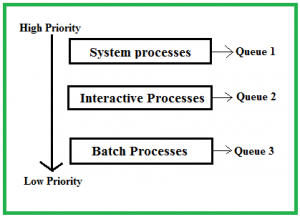
1. High-Priority Queue: This queue contains processes that are of high importance or require immediate attention. For instance, real-time tasks or system processes.
2. Medium-Priority Queue: This might contain regular processes or interactive tasks.
3. Low-Priority Queue: This queue holds background or batch processes that are less time-sensitive.

Example

Consider a system with three queues:

1. Queue 1 (High Priority): Uses Round Robin (RR) scheduling.
2. Queue 2 (Medium Priority): Uses Shortest Job First (SJF) scheduling.
3. Queue 3 (Low Priority): Uses First-Come, First-Served (FCFS) scheduling.

Suppose we have the following processes:

• Process P1: Arrival Time = 0, Burst Time = 10 units, Assigned to Queue 1
• Process P2: Arrival Time = 2, Burst Time = 5 units, Assigned to Queue 2
• Process P3: Arrival Time = 4, Burst Time = 8 units, Assigned to Queue 3

Scheduling Process

1. Queue 1 (RR Scheduling): P1 is processed first using Round Robin.
2. Queue 2 (SJF Scheduling): P2 is processed next based on Shortest Job First.
3. Queue 3 (FCFS Scheduling): P3 is processed last using First-Come, First-Served.

Execution Order

1. Queue 1: P1 starts executing from time 0 to 4 units (assuming a time quantum of 4 units). It resumes after processing of Queue 2 and Queue 3.
2. Queue 2: P2 arrives at time 2 and starts executing after Queue 1 processes time quantum. P2 completes at time 7.
3. Queue 3: P3 starts executing after Queue 2 and completes at time 15.
4. Queue 1: Resumes with P1 and completes its execution from time 15 to 18.

Gantt Chart:

| P1 | P2 | P3 | P1 |
|----|----|----|----|
| 0  | 4  | 7  | 15 | 18

Waiting Time Calculation

• Process P1:
  • Wait time before first execution = 0 units.
  • Wait time during second execution = (7 – 4) = 3 units.
  • Wait time during third execution = (15 – 7) = 8 units.
  • Total wait time = 3 + 8 = 11 units.
• Process P2:
  • Wait time before execution = 2 units (waits for Queue 1 processing).
  • Total wait time = 2 units.
• Process P3:
  • Wait time before execution = 4 units (waits for Queue 1 and Queue 2 processing).
  • Total wait time = 4 units.

Average Waiting Time:(11+2+4)3=173=5.67 units\frac{(11 + 2 + 4)}{3} = \frac{17}{3} = 5.67 \text{ units}3(11+2+4)​=317​=5.67 units

Advantages of Multilevel Queue Scheduling

1. Prioritization: Different queues allow the system to prioritize processes based on their importance and type.
2. Flexibility: Each queue can use a different scheduling algorithm suitable for its type of processes.
3. Efficiency: Can be tuned to optimize for different types of processes and workloads.

Disadvantages of Multilevel Queue Scheduling

1. Complexity: Managing multiple queues and their scheduling algorithms can be complex.
2. Fixed Queue Assignment: Processes are typically assigned to a specific queue at creation, making it difficult to adapt dynamically if the process’s behavior changes.
3. Potential for Starvation: Lower-priority queues may suffer from starvation if higher-priority queues are always busy.

Real-Life Example

Scenario: A customer service center uses a multilevel queue system to manage support requests.

1. Queue 1 (High Priority): Urgent technical issues that need immediate attention (e.g., system outages).
2. Queue 2 (Medium Priority): Routine technical support (e.g., software bugs or issues).
3. Queue 3 (Low Priority): General inquiries or non-urgent issues (e.g., product information requests).

Execution

• High Priority requests are handled first, ensuring that critical issues are resolved quickly.
• Medium Priority requests are handled next, focusing on less urgent but still important support needs.
• Low Priority requests are addressed last, dealing with non-urgent inquiries.

Conclusion

Multilevel Queue Scheduling is effective for systems with diverse types of processes or tasks that need different handling priorities. It balances the workload based on priority, ensuring that critical tasks receive timely attention while managing less urgent tasks efficiently.

6.Multilevel Feedback Queue Scheduling

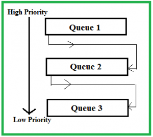
Multilevel Feedback Queue (MLFQ) Scheduling is an advanced version of the multilevel queue scheduling algorithm. It combines the concepts of multiple queues with dynamic feedback mechanisms to adapt to varying process behaviors over time. The key feature of MLFQ is that processes can move between different queues based on their behavior, which allows the system to better handle processes with varying requirements.

Key Features

1. Multiple Queues: Similar to multilevel queue scheduling, MLFQ uses multiple queues with different priority levels.
2. Dynamic Adjustment: Processes can move between queues based on their behavior and CPU usage.
3. Feedback Mechanism: The system adjusts the priority of processes dynamically based on their execution patterns.

Operation

1. Initial Queue Assignment: When a process starts, it is placed in the highest priority queue.
2. Time Quantum: Each queue has a different time quantum. The highest priority queue usually has a shorter time quantum, while lower-priority queues have longer time quanta.
3. Feedback: If a process uses up its time quantum without completing, it is moved to a lower-priority queue. If it completes before its time quantum expires, it can be moved back to a higher-priority queue or remain in the current queue.
4. Promotion and Demotion: Processes that are preempted or use excessive CPU time are demoted to lower-priority queues, while processes that complete quickly or use less CPU time can be promoted to higher-priority queues.

Example

Consider a system with three queues:

1. Queue 1 (High Priority): Time Quantum = 2 units
2. Queue 2 (Medium Priority): Time Quantum = 4 units
3. Queue 3 (Low Priority): Time Quantum = 6 units

Processes:

• Process P1: Arrival Time = 0, Burst Time = 10 units
• Process P2: Arrival Time = 2, Burst Time = 6 units
• Process P3: Arrival Time = 4, Burst Time = 8 units

Execution Order with MLFQ:

1. Queue 1: Processes P1, P2, and P3 start in Queue 1.
   • P1 runs from time 0 to 2 units, gets demoted to Queue 2.
   • P2 runs from time 2 to 4 units, also gets demoted to Queue 2.
   • P3 starts at time 4, runs from 4 to 6 units, and gets demoted to Queue 2.
2. Queue 2: Processes P1, P2, and P3 continue in Queue 2.
   • P1 resumes at time 6, runs from 6 to 10 units, and completes.
   • P2 resumes at time 10, runs from 10 to 14 units, and completes.
   • P3 resumes at time 14, runs from 14 to 20 units, and completes.

Gantt Chart:

| P1 | P2 | P3 | P1 | P2 | P3 |
|----|----|----|----|----|----|
| 0  | 2  | 4  | 6  | 10 | 14 | 20

Waiting Time Calculation

• Process P1:
  • Waiting time before execution = 0 units.
  • Wait time between Queue 1 and Queue 2 = (6 – 2) = 4 units.
  • Total wait time = 4 units.
• Process P2:
  • Waiting time before execution = 2 units.
  • Wait time between Queue 1 and Queue 2 = (10 – 4) = 6 units.
  • Total wait time = 2 + 6 = 8 units.
• Process P3:
  • Waiting time before execution = 4 units.
  • Wait time between Queue 2 and completion = (14 – 6) = 8 units.
  • Total wait time = 4 + 8 = 12 units.

Average Waiting Time:(4+8+12)3=243=8 units\frac{(4 + 8 + 12)}{3} = \frac{24}{3} = 8 \text{ units}3(4+8+12)​=324​=8 units

Advantages of Multilevel Feedback Queue Scheduling

1. Adaptive: Adapts to the behavior of processes, handling both short and long processes efficiently.
2. Fairness: Provides better responsiveness for interactive processes while preventing long processes from monopolizing the CPU.
3. Flexibility: Dynamic adjustment of priorities allows for more efficient CPU utilization.

Disadvantages of Multilevel Feedback Queue Scheduling

1. Complexity: Managing multiple queues and dynamic adjustments can be complex and resource-intensive.
2. Starvation: Although MLFQ aims to prevent starvation, low-priority processes can still experience delays if higher-priority processes continuously arrive.
3. Tuning: Choosing the appropriate number of queues and time quanta requires careful tuning to balance performance and responsiveness.

Real-Life Example

Scenario: A printing system that handles various types of print jobs with different priorities.

1. Queue 1 (High Priority): Jobs requiring immediate printing, such as emergency reports.
2. Queue 2 (Medium Priority): Regular print jobs, such as office documents.
3. Queue 3 (Low Priority): Non-urgent print jobs, such as large batch print requests.

Execution:

• High Priority jobs are printed first, ensuring that urgent documents are handled quickly.
• Medium Priority jobs are printed next, balancing efficiency and fairness.
• Low Priority jobs are handled last, ensuring that large or non-urgent jobs do not delay more critical tasks.

Feedback Mechanism:

• If a high-priority job is not completed within its time quantum, it may be demoted to a lower-priority queue if it’s a large batch job or if the system is overloaded.
• Conversely, if a low-priority job completes quickly, it may be promoted to a higher-priority queue for faster handling in the future.

Conclusion

Multilevel Feedback Queue Scheduling provides a dynamic and flexible approach to process management by adapting to process behaviors and priorities. It balances responsiveness and fairness, making it suitable for systems with diverse workloads and varying process requirements. However, its complexity and the need for careful tuning can pose challenges in practical implementations.