
Introduction of Non-linear Data structures
Non-linear data structures are types of data structures where elements are not arranged in a sequential order. Unlike linear data structures such as arrays, linked lists, stacks, and queues, non-linear data structures do not follow a sequential order and instead have a hierarchical or interconnected arrangement of elements. This allows for more complex relationships between elements, and they are used to represent various real-world problems and scenarios efficiently.
Advantages of Non-linear Data Structures
- Hierarchical Representation: Trees represent hierarchical relationships, making them suitable for problems like organizational structures, file systems, and decision-making processes.
- Efficient Searching and Sorting: Trees and heaps allow for efficient searching, insertion, and deletion operations, especially in dynamic datasets.
- Model Complex Relationships: Graphs are ideal for modeling complex relationships in networks, such as social networks, communication networks, and transportation systems.
- Flexibility: Non-linear structures like graphs can represent various types of connections and relationships between elements, providing flexibility in problem-solving.
Common Operations
- Tree Operations:
- Traversal: In-order, pre-order, post-order traversals.
- Insertion: Adding nodes while maintaining tree properties.
- Deletion: Removing nodes and restructuring the tree if necessary.
- Searching: Finding nodes or values based on specific criteria.
- Graph Operations:
- Traversal: Breadth-First Search (BFS) and Depth-First Search (DFS).
- Shortest Path: Algorithms like Dijkstra’s and Bellman-Ford for finding the shortest path between nodes.
- Connectivity: Checking if all nodes are connected (e.g., connected components).
- Heap Operations:
- Insertion: Adding elements while maintaining the heap property.
- Deletion: Removing the root element and re-adjusting the heap.
- Peek: Accessing the root element without removal.
Summary
Non-linear data structures, including trees, graphs, and heaps, offer powerful ways to model and solve complex problems by representing relationships and hierarchies that linear structures cannot efficiently handle. They are fundamental in various applications ranging from database indexing and network design to computational algorithms and real-world systems modeling.
Trees
A tree is a non-linear data structure that represents hierarchical relationships among elements. It consists of nodes connected by edges, and each node can have zero or more child nodes. Trees are fundamental in computer science and are used in various applications such as file systems, databases, and network protocols.
Example: Binary Search Tree (BST)
A Binary Search Tree (BST) is a type of binary tree where each node follows these rules:
- The left child’s value is less than the node’s value.
- The right child’s value is greater than the node’s value.
Here’s an example of a BST:
       50
       /  \
      30   70
     / \   / \
    20 40 60 80
Explanation
- Root: The root node is 50.
- Nodes: Each node contains a value and links to other nodes. For instance, the node with value 30 has two children: 20 and 40.
- Leaf Nodes: The leaf nodes in this tree are 20, 40, 60, and 80. They have no children.
- Parent Nodes: For example, the node with value 30 is a parent to nodes 20 and 40.
- Subtree: The subtree rooted at node 30 includes nodes 20, 30, and 40.
- Height: The height of the node with value 50 is 2 (the longest path to a leaf is 2 edges long).
Tree Operations
- Insertion
- Insert 25: To insert a new value into the BST, we start from the root and compare the value to be inserted with the current node’s value. If it’s less, we move to the left child; if greater, we move to the right child. If we find an appropriate spot (where the child is null), we insert the new value there.
- Deletion
- Delete 30: To delete a node, we need to handle three cases:
- Node to be deleted has no children: Simply remove the node.
- Node to be deleted has one child: Replace the node with its child.
- Node to be deleted has two children: Find the node’s in-order successor (the smallest node in the right subtree), replace the node with its in-order successor, and then delete the in-order successor.
- Delete 30: To delete a node, we need to handle three cases:
- Traversal
- In-order Traversal: Visit the left subtree, then the node, then the right subtree. For the example BST, in-order traversal would yield: 20, 25, 30, 40, 50, 60, 70, 80.
- Pre-order Traversal: Visit the node first, then the left subtree, then the right subtree. For the example BST, pre-order traversal would yield: 50, 30, 20, 40, 70, 60, 80.
- Post-order Traversal: Visit the left subtree, then the right subtree, then the node. For the example BST, post-order traversal would yield: 20, 40, 30, 60, 80, 70, 50.
- Searching
- Search for 60: Starting from the root, compare the value 60 with the current node. If it’s less, move to the left child; if greater, move to the right child. Continue until the node is found or a leaf is reached.
Summary
Trees are essential data structures used for hierarchical representation and efficient data management. In a Binary Search Tree (BST), data is organized in a way that makes searching, insertion, and deletion operations efficient. Understanding tree operations and their applications is crucial for solving complex problems in computer science.
Terminology Related to tree
1. Node
- Definition: A node is the fundamental component of a tree structure. It contains data and may have links (or pointers) to other nodes.
- example
    A
   / \
  B   C
 / \
D   E
Here, A, B, C, D, and E are nodes. Each node contains data and can have links to child nodes. For instance, node A contains data and has pointers to nodes B and C.
2. Edge
- Definition: An edge is the connection or link between two nodes. It represents the relationship or path between nodes in a tree.
- Example:
    A
   / \
  B   C
 / \
D   E
The edges are A-B, A-C, B-D, and B-E. These edges connect the nodes, showing the hierarchy or relationship between them. For instance, A-B indicates that node B is a child of node A.
3. Root
- Definition: The root is the topmost node of a tree. It is the starting point of the tree and does not have a parent. All other nodes are descendants of the root.
- Example:
    A
   / \
  B   C
 / \
D   E
Node A is the root of this tree. It is the entry point of the tree structure and serves as the origin from which all other nodes descend.
4. Leaf
- Definition: A leaf is a node that has no children. It is located at the end of a branch in the tree and does not point to any other nodes.
- Example
    A
   / \
  B   C
 / \
D   E
Nodes D and E are leaves because they do not have any child nodes.
5. Parent
- Definition: A parent is a node that has one or more child nodes. It represents the direct predecessor in the hierarchy for its children.
- Example:
    A
   / \
  B   C
 / \
D   E
Node A is the parent of nodes B and C. Node B is the parent of nodes D and E. Parents are nodes from which other nodes (children) branch out.
6. Child
- Definition: A child is a node that is directly connected to another node (its parent). It represents a node that is one level below its parent.
- Example:
    A
   / \
  B   C
 / \
D   E
Nodes B and C are children of node A. Nodes D and E are children of node B. Children are the nodes that branch out from a parent.
7. Subtree
- Definition: A subtree is a portion of a tree that consists of a node and all its descendants. It forms a tree within the original tree.
- Example
    A
   / \
  B   C
 / \
D   E
The subtree rooted at node B includes nodes B, D, and E. It represents a smaller tree structure within the larger tree starting at node B.
8. Height
- Definition: The height of a node is the length of the longest path from that node to any of its leaf nodes. The height of a leaf node is 0.
- Example
    A
   / \
  B   C
 / \
D   E
The height of node D is 0 (since it is a leaf).
The height of node B is 1 (longest path to leaf D has 1 edge).
The height of node A is 2 (longest path to leaf D is through B and D, which has 2 edges).
9. Depth
- Definition: The depth of a node is the number of edges from the root to that node. It reflects how far the node is from the root. The root node has a depth of 0.
- Example:
    A
   / \
  B   C
 / \
D   E
The depth of node A (root) is 0.
The depth of node B is 1.
The depth of node D is 2.
10. Level
 Definition: The level of a node is the depth of the node plus one. It represents the node’s distance from the root, where the root is at level 1.
Example:
      A
     / \
    B   C
   / \
  D   E
  ```
  - The level of node `A` is 1.
  - The level of nodes `B` and `C` is 2.
  - The level of nodes `D` and `E` is 3.
11. Forest
- Definition: A forest is a collection of disjoint trees. Essentially, it is a set of trees that do not share any nodes or edges with each other. Each tree in the forest is an individual tree with its own structure and properties.
- Example
   Tree 1:         Tree 2:
       A              P
      / \            / \
     B   C          Q   R
    /              / \
   D              S   T
In this example, the two trees (Tree 1 and Tree 2) together form a forest. They are separate and do not overlap in any way.
12. Degree
- Definition: The degree of a node in a tree is the number of children it has. In other words, it represents how many direct connections (child nodes) a node has.
- Example
    A
   /|\
  B C D
 / \
E   F
Node A has a degree of 3 (children are B, C, and D).
Node B has a degree of 2 (children are E and F).
Nodes C, D, E, and F have a degree of 0 (they are leaves with no children).
13. Siblings
- Definition: Siblings are nodes that share the same parent. In other words, they are children of the same parent node.
- Example
    A
   /|\
  B C D
 / \
E   F
Nodes B, C, and D are siblings because they all share the same parent node A.
Nodes E and F are siblings because they share the same parent node B.
Binary Tree
Definition
A binary tree is a type of tree data structure in which each node has at most two children. These children are typically referred to as the left child and the right child. Binary trees are fundamental in computer science and are used to implement various data structures and algorithms.
Properties
- Each node has at most two children:
- A node in a binary tree can have either 0, 1, or 2 children.
- Hierarchical Structure:
- The binary tree has a hierarchical structure with a root node at the top and nodes below it arranged in levels.
- Subtrees:
- Each node in a binary tree forms the root of a subtree. The entire tree is itself a subtree of the root node.
- Example:
    1
   / \
  2   3
 / \ / \
4  5 6  7
Here, all nodes have two children, and all leaf nodes are at the same level.
Summary
A binary tree is a versatile data structure where each node has at most two children, with various types and properties tailored to different applications. Understanding its traversal methods and types helps in efficiently implementing and managing hierarchical data.
Difference Between General tree and Binary Tree
| Aspect | General Tree | Binary Tree |
|---|---|---|
| Definition | A tree where each node can have any number of children. | A tree where each node has at most two children (left and right). |
| Number of Children | Each node can have 0 or more children. | Each node can have 0, 1, or 2 children. |
| Children Classification | No specific classification for children. | Children are classified as left child and right child. |
| Tree Structure | More flexible; nodes can have varying numbers of children. | More rigid; each node strictly has 0, 1, or 2 children. |
| Example | A/|\ B C D /|\ E F G | A/ \ B C / \ D E |
| Traversal Methods | Can be traversed in various ways depending on tree structure (pre-order, post-order, etc.). | Commonly uses in-order, pre-order, post-order, and level-order traversals. |
| Use Cases | Used in hierarchical data structures where nodes can have varying numbers of sub-items (e.g., file systems). | Used for applications requiring efficient searching, sorting, and hierarchical data representation (e.g., binary search trees, heaps). |
| Subtree Definition | Any node and its descendants form a subtree. | Any node and its left and right subtrees form a subtree. |
| Complexity | Can be more complex due to varying number of children and tree structure. | Typically simpler due to the constraint of at most two children per node. |
Conversion of General Trees to Binary tree
Converting a general tree to a binary tree involves transforming the structure of the general tree to fit the binary tree constraints, where each node can have at most two children. This conversion is typically achieved using a method called the left-child, right-sibling representation. Here’s a step-by-step explanation of the conversion process:
Conversion Process: Left-Child, Right-Sibling Representation
Concept
In the left-child, right-sibling representation, each node in the general tree is represented as a node in the binary tree:
- The left child of a binary tree node corresponds to the first child of the general tree node.
- The right child of a binary tree node corresponds to the next sibling of the general tree node.
Steps for Conversion
- Initialize the Binary Tree:
- Create a new binary tree where each node will represent a node from the general tree.
- Assign the Left Child:
- For each node in the general tree, the left child in the binary tree will be the first child of the general tree node.
- Assign the Right Sibling:
- For each node, the right child in the binary tree will be the next sibling of the general tree node.
- Recursively Apply the Conversion:
- Apply the same conversion recursively for the left child and right child nodes.
Examples:
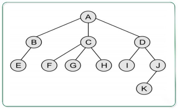
Convert the following Generic Tree to Binary Tree:
steps to convert binary tree
Note: If the parent node has only the right child in the general tree then it becomes the rightmost child node of the last node following the parent node in the binary tree. In the above example, if node B has the right child node L then in binary tree representation L would be the right child of node D.
Below are the steps for the conversion of Generic Tree to Binary Tree:
- As per the rules mentioned above, the root node of general tree A is the root node of the binary tree.
- Now the leftmost child node of the root node in the general tree is B and it is the leftmost child node of the binary tree.
- Now as B has E as its leftmost child node, so it is its leftmost child node in the binary tree whereas it has C as its rightmost sibling node so it is its right child node in the binary tree.
- Now C has F as its leftmost child node and D as its rightmost sibling node, so they are its left and right child node in the binary tree respectively.
- Now D has I as its leftmost child node which is its left child node in the binary tree but doesn’t have any rightmost sibling node, so doesn’t have any right child in the binary tree.
- Now for I, J is its rightmost sibling node and so it is its right child node in the binary tree.
- Similarly, for J, K is its leftmost child node and thus it is its left child node in the binary tree.
- Now for C, F is its leftmost child node, which has G as its rightmost sibling node, which has H as its just right sibling node and thus they form their left, right, and right child node respectively.
Linear Representation and Linked list Representation of a Binary tree
Linear Representation (Array)
Definition: In the linear representation of a binary tree, the tree is stored in a contiguous block of memory (i.e., an array). Each node’s position in the array is determined by its position in the tree. The root node is at index 0, the left child of a node at index i is at index 2*i + 1, and the right child is at index 2*i + 2.
Linked List Representation
Definition: In the linked list representation of a binary tree, each node is represented by a structure (or object) that contains a data element and pointers (or references) to its left and right children. This representation allows for dynamic tree structures where nodes can be added or removed easily.
Binary search tree
Definition
A Binary Search Tree (BST) is a type of binary tree where each node has at most two children, and it maintains the following property:
- For any node:
- The value of all nodes in its left subtree is less than the value of the node.
- The value of all nodes in its right subtree is greater than the value of the node.
This property ensures that the BST is sorted and enables efficient searching, insertion, and deletion operations.
Properties
- In-Order Traversal:
- The in-order traversal of a BST produces a sorted sequence of values.
- Search Time Complexity:
- On average, searching for a value in a BST has a time complexity of O(log n), where
nis the number of nodes, assuming the tree is balanced.
- On average, searching for a value in a BST has a time complexity of O(log n), where
- Insertion and Deletion:
- Insertion and deletion operations also have an average time complexity of O(log n) if the tree is balanced.
- Balance:
- The efficiency of a BST depends on its balance. An unbalanced BST may degrade to a linear structure (like a linked list) in the worst case.
Example:
    8
   / \
  3   10
 / \    \
1   6    14
   / \   /
  4   7  13
Root Node: 8
Left Subtree of 8:
- Root:
3 - Left Subtree:
1 - Right Subtree:
6(with children4and7)
Right Subtree of 8:
- Root:
10 - Right Subtree:
14(with child13)
Difference Between Binary Search Tree and Binary Tree
| Aspect | Binary Search Tree (BST) | Binary Tree |
|---|---|---|
| Definition | A binary tree where each node has at most two children, and the left child’s value is less than the node’s value, and the right child’s value is greater. | A tree where each node has at most two children, with no specific ordering constraint on the values. |
| Ordering | Nodes are arranged according to their values, with the left subtree containing values less than the node’s value and the right subtree containing values greater. | No specific ordering; nodes can be arranged in any manner. |
| Search Efficiency | Search operations are efficient (O(log n) on average) due to the ordering, making it easier to find values quickly. | Search operations are generally less efficient (O(n)) because there is no ordering to aid in the search. |
| Insertion Efficiency | Insertion is efficient (O(log n) on average) when the tree is balanced, due to the ordered structure. | Insertion is less efficient (O(n)) since the tree lacks ordering, requiring traversal to find the insertion point. |
| Deletion Efficiency | Deletion is more complex and involves cases depending on the node’s number of children, but remains efficient (O(log n) on average) with a balanced tree. | Deletion is simpler but less efficient (O(n)) due to the lack of structure. |
| Traversal | In-order traversal of a BST results in a sorted sequence of values. | Traversal methods (in-order, pre-order, post-order) do not guarantee a sorted sequence. |
| Example | 8 <br> / \ <br> 3 10 <br> / \ <br> 1 6 <br> / \ <br> 4 7 | 8 <br> / \ <br> 3 10 <br> / \ <br> 1 6 <br> / \ <br> 4 7 |
| Applications | Used in applications that require fast search, insertion, and deletion, such as databases and memory management. | Used in more general applications where hierarchical data is managed, such as expression trees and file systems. |
| Balance | A BST can be balanced or unbalanced; balance affects efficiency. Variants like AVL trees or Red-Black trees maintain balance for better performance. | A binary tree can be balanced or unbalanced, but there is no inherent balancing requirement. |
Various Traversals on Binary Search Tree
1.In-Order Traversal:
- Description: Visit the left subtree, the current node, and then the right subtree.
- Order: Left, Root, Right
- Purpose: It produces a sorted sequence of values for a BST.
- Algorithm:
- Traverse the left subtree.
- Visit the root node.
- Traverse the right subtree.
- Example:
   10
  /  \
 5    20
/ \   / \
3  8 15 25
In-Order Traversal
Algorithm: Left, Root, Right
- Traverse left subtree of 10:
- Traverse left subtree of 5:
- Traverse left subtree of 3 (no left child).
- Visit 3.
- Traverse right subtree of 3 (no right child).
- Visit 5.
- Traverse right subtree of 5:
- Traverse left subtree of 8 (no left child).
- Visit 8.
- Traverse right subtree of 8 (no right child).
- Traverse left subtree of 5:
- Visit 10.
- Traverse right subtree of 10:
- Traverse left subtree of 20:
- Traverse left subtree of 15 (no left child).
- Visit 15.
- Traverse right subtree of 15 (no right child).
- Visit 20.
- Traverse right subtree of 20:
- Traverse left subtree of 25 (no left child).
- Visit 25.
- Traverse right subtree of 25 (no right child).
- Traverse left subtree of 20:
In-Order Traversal Result: 3, 5, 8, 10, 15, 20, 25
2.Pre-Order Traversal:
- Description: Visit the current node before its child nodes.
- Order: Root, Left, Right
- Purpose: Useful for creating a prefix expression or for cloning the tree.
- Algorithm:
- Visit the root node.
- Traverse the left subtree.
- Traverse the right subtree.
- Example:
   10
  /  \
 5    20
/ \   / \
3 8 15 25
Pre-Order Traversal
Algorithm: Root, Left, Right
- Visit 10.
- Traverse left subtree of 10:
- Visit 5.
- Traverse left subtree of 5:
- Visit 3.
- Traverse right subtree of 5:
- Visit 8.
- Traverse right subtree of 10:
- Visit 20.
- Traverse left subtree of 20:
- Visit 15.
- Traverse right subtree of 20:
- Visit 25.
3.Pre-Order Traversal Result: 10, 5, 3, 8, 20, 15, 25
3.Post-Order Traversal:
- Description: Visit the current node after its child nodes.
- Order: Left, Right, Root
- Purpose: Useful for deleting or freeing nodes, or evaluating postfix expressions.
- Algorithm:
- Traverse the left subtree.
- Traverse the right subtree.
- Visit the root node.
- Example:
   10
  /  \
 5    20
/ \   / \
3 8 15 25Algorithm: Left, Right, Root
- Traverse left subtree of 10:
- Traverse left subtree of 5:
- Traverse left subtree of 3 (no left child).
- Traverse right subtree of 3 (no right child).
- Visit 3.
- Traverse right subtree of 5:
- Traverse left subtree of 8 (no left child).
- Traverse right subtree of 8 (no right child).
- Visit 8.
- Visit 5.
- Traverse left subtree of 5:
- Traverse right subtree of 10:
- Traverse left subtree of 20:
- Traverse left subtree of 15 (no left child).
- Traverse right subtree of 15 (no right child).
- Visit 15.
- Traverse right subtree of 20:
- Traverse left subtree of 25 (no left child).
- Traverse right subtree of 25 (no right child).
- Visit 25.
- Visit 20.
- Traverse left subtree of 20:
- Visit 10.
Construct a Binary Tree using In-order and Pre-Order Traversals
To construct a Binary Tree from given In-Order and Pre-Order traversals, you can follow these steps:
- Understand the Traversals:
- In-Order Traversal: This traversal lists nodes in the order of left subtree, root, right subtree.
- Pre-Order Traversal: This traversal lists nodes in the order of root, left subtree, right subtree.
- Build the Tree:
- Step 1: The first element of the Pre-Order traversal is the root of the tree.
- Step 2: Find this root in the In-Order traversal. Elements to the left of this root in the In-Order traversal belong to the left subtree, and elements to the right belong to the right subtree.
- Step 3: Recursively repeat the process for the left and right subtrees using the corresponding elements from the In-Order and Pre-Order traversals.
Example
Let’s use the following traversals:
- In-Order Traversal:
D, B, E, A, F, C - Pre-Order Traversal:
A, B, D, E, C, F
Step-by-Step Construction:
- Identify the Root:
- From the Pre-Order traversal, the first element is
A. So,Ais the root of the tree.
- From the Pre-Order traversal, the first element is
- Split the In-Order Traversal:
- Find
Ain the In-Order traversal:D, B, E, A, F, C - Elements to the left of
A(D, B, E) are part of the left subtree. - Elements to the right of
A(F, C) are part of the right subtree.
- Find
- Construct the Left Subtree:
- For the left subtree, use the In-Order part
D, B, Eand the next elements in the Pre-Order traversal (B, D, E):- The root of this subtree is
B(the first element in the Pre-Order traversal for this subtree). - Find
BinD, B, E. Elements to the left ofB(D) are part of the left subtree ofB, and elements to the right ofB(E) are part of the right subtree ofB. - For the left subtree of
B, use In-OrderDand Pre-OrderD.Dis a leaf node.
- For the right subtree of
B, use In-OrderEand Pre-OrderE.Eis a leaf node.
- The root of this subtree is
- For the left subtree, use the In-Order part
- Construct the Right Subtree:
- For the right subtree, use the In-Order part
F, Cand the next elements in the Pre-Order traversal (C, F):- The root of this subtree is
C(the first element in the Pre-Order traversal for this subtree). - Find
CinF, C. Elements to the left ofC(F) are part of the left subtree ofC. - For the left subtree of
C, use In-OrderFand Pre-OrderF.Fis a leaf node.
- The root of this subtree is
- For the right subtree, use the In-Order part
Resulting Tree Structure:
        A
       / \
      B   C
     / \   \
    D   E   F
Summary
To reconstruct a Binary Tree from In-Order and Pre-Order traversals:
- Identify the root from the Pre-Order traversal.
- Divide the In-Order traversal into left and right subtrees around the root.
- Recursively apply the same steps to the left and right subtrees using the corresponding segments of the In-Order and Pre-Order traversals.
Construct a Binary Tree using In-order and Post Order Traversals
To construct a Binary Tree from given In-Order and Post-Order traversals, follow these steps:
- Understand the Traversals:
- In-Order Traversal: Lists nodes in the order of left subtree, root, right subtree.
- Post-Order Traversal: Lists nodes in the order of left subtree, right subtree, root.
- Build the Tree:
- Step 1: The last element of the Post-Order traversal is the root of the tree.
- Step 2: Find this root in the In-Order traversal. Elements to the left of this root in the In-Order traversal belong to the left subtree, and elements to the right belong to the right subtree.
- Step 3: Recursively repeat the process for the left and right subtrees using the corresponding elements from the In-Order and Post-Order traversals.
Example
Let’s use the following traversals:
- In-Order Traversal:
D, B, E, A, F, C - Post-Order Traversal:
D, E, B, F, C, A
Step-by-Step Construction:
- Identify the Root:
- From the Post-Order traversal, the last element is
A. So,Ais the root of the tree.
- From the Post-Order traversal, the last element is
- Split the In-Order Traversal:
- Find
Ain the In-Order traversal:D, B, E, A, F, C - Elements to the left of
A(D, B, E) are part of the left subtree. - Elements to the right of
A(F, C) are part of the right subtree.
- Find
- Construct the Left Subtree:
- For the left subtree, use the In-Order part
D, B, Eand the Post-Order partD, E, B:- The root of this subtree is
B(the last element in the Post-Order traversal for this subtree). - Find
BinD, B, E. Elements to the left ofB(D) are part of the left subtree ofB, and elements to the right ofB(E) are part of the right subtree ofB. - For the left subtree of
B, use In-OrderDand Post-OrderD.Dis a leaf node.
- For the right subtree of
B, use In-OrderEand Post-OrderE.Eis a leaf node.
- The root of this subtree is
- For the left subtree, use the In-Order part
- Construct the Right Subtree:
- For the right subtree, use the In-Order part
F, Cand the Post-Order partF, C:- The root of this subtree is
C(the last element in the Post-Order traversal for this subtree). - Find
CinF, C. Elements to the left ofC(F) are part of the left subtree ofC. - For the left subtree of
C, use In-OrderFand Post-OrderF.Fis a leaf node.
- The root of this subtree is
- For the right subtree, use the In-Order part
Resulting Tree Structure:
        A
       / \
      B   C
     / \   \
    D   E   F
Summary
To reconstruct a Binary Tree from In-Order and Post-Order traversals:
- Identify the root from the Post-Order traversal.
- Divide the In-Order traversal into left and right subtrees around the root.
- Recursively apply the same steps to the left and right subtrees using the corresponding segments of the In-Order and Post-Order traversals.
Importance of Binary Search Trees over General Trees
1. Efficient Search, Insertion, and Deletion
- BSTs: In a balanced BST (e.g., AVL Tree, Red-Black Tree), operations such as search, insertion, and deletion have a time complexity of O(logn)O(\log n)O(logn), where nnn is the number of nodes. This is due to the tree’s property where each node’s left child contains smaller values, and the right child contains larger values.
- General Trees: For general trees, these operations can take O(n)O(n)O(n) in the worst case because you might need to traverse the entire tree.
2. Sorted Data
- BSTs: In an in-order traversal of a BST, the nodes are visited in sorted order. This property makes it easy to retrieve data in a sorted manner without needing extra sorting operations.
- General Trees: General trees do not guarantee any particular order among their nodes, so additional effort is required to sort or retrieve data in a specific order.
3. Efficient Range Queries
- BSTs: Range queries (e.g., finding all values between two given numbers) are efficient in BSTs because you can traverse only the relevant parts of the tree, leveraging the ordering property.
- General Trees: Range queries in general trees can be less efficient because they might require examining all nodes.
4. Dynamic Data Structure
- BSTs: BSTs support dynamic updates, such as inserting and deleting nodes, efficiently while maintaining their ordering properties.
- General Trees: While general trees can also be dynamic, maintaining specific order or properties during updates can be more complex and less efficient.
5. Balanced BST Variants
- Balanced BSTs: Variants like AVL Trees and Red-Black Trees maintain balance, ensuring that the tree remains approximately balanced. This helps keep operations efficient even as the tree grows.
- General Trees: General trees do not inherently provide balancing mechanisms, which can lead to inefficient operations if the tree becomes unbalanced.
6. Space Complexity
- BSTs: Space complexity is O(n)O(n)O(n) for a BST, where nnn is the number of nodes, and each node has a fixed number of children (two).
- General Trees: Space complexity can also be O(n)O(n)O(n), but the tree’s structure can vary greatly, potentially leading to more complex storage and management overhead.
7. Use Cases
- BSTs: Ideal for applications requiring fast lookups, ordered data retrieval, and efficient management of dynamic datasets, such as in-memory databases, file systems, and indexing systems.
- General Trees: Useful for representing hierarchical structures that do not require ordering, such as organizational charts, file directory structures, and XML/HTML document trees.
Summary
Binary Search Trees provide efficient searching, insertion, and deletion operations due to their ordering properties, making them suitable for applications that need ordered data and quick access. General trees are more flexible in representing complex hierarchical structures but do not inherently offer the same efficiency for ordered operations and queries.
Perform Insertion , Deletion , Search , and Various Traversal Operations on a Binary Search tree
1. Insertion
To insert a new node in a BST, follow these steps:
- Step 1: Start at the root.
- Step 2: Compare the new value with the current node’s value.
- If the new value is less, move to the left child.
- If the new value is greater, move to the right child.
- Step 3: Repeat until you find a suitable empty spot for the new node.
- Example:
   50
  /  \
 30   70
/ \   / \
20 40 60 80Example: Insert 65 into the BST.
- Start at
50(root):65is greater, move to the right child (70). - At
70:65is less, move to the left child (60). - At
60:65is greater, so insert65as the right child of60.
Updated BST:
       50
      /  \
     30   70
    / \   / \
   20 40 60 80
        \
        65
2. Deletion
To delete a node from a BST, follow these steps:
- Step 1: Locate the node to delete.
- Step 2: Handle three possible cases:
- Case 1: Node has no children (leaf node). Simply remove it.
- Case 2: Node has one child. Remove the node and replace it with its child.
- Case 3: Node has two children. Find the node’s in-order successor (smallest node in the right subtree), replace the node’s value with the successor’s value, and delete the successor.
- Example:
   50
  /  \
 30   70
/ \   / \
20 40 60 80Example: Delete 70 from the BST.
- Start at
50:70is greater, move to the right child (70). - Node
70has two children. Find the in-order successor (80in this case) and replace70with80. - Remove
80, which is a leaf node.
Updated BST:
       50
      /  \
     30   80
    / \   /
   20 40 60
        \
        65
3. Search
To search for a value in a BST:
- Step 1: Start at the root.
- Step 2: Compare the target value with the current node’s value.
- If equal, the node is found.
- If less, move to the left child.
- If greater, move to the right child.
- Step 3: Repeat until you find the node or reach a leaf node (if not found).
- Example:
       50
      /  \
     30   70
    / \   / \
   20 40 60 80
Search for 65.
- Start at
50:65is greater, move to the right child (80). - At
80:65is less, move to the left child (60). - At
60:65is greater, move to the right child (65). - Found
65.
program for Binary Search Tree with all operations
#include <stdio.h>
#include <stdlib.h>

// Definition of a node in the BST
typedef struct Node {
    int data;
    struct Node* left;
    struct Node* right;
} Node;

// Function prototypes
Node* createNode(int data);
Node* insert(Node* root, int data);
Node* deleteNode(Node* root, int data);
Node* search(Node* root, int data);
Node* findMin(Node* root);

int main() {
    Node* root = NULL;

    // Inserting nodes
    root = insert(root, 50);
    root = insert(root, 30);
    root = insert(root, 70);
    root = insert(root, 20);
    root = insert(root, 40);
    root = insert(root, 60);
    root = insert(root, 80);

    // Search for a value
    int value = 60;
    Node* result = search(root, value);
    if (result) {
        printf("Node %d found in the BST.\n", value);
    } else {
        printf("Node %d not found in the BST.\n", value);
    }

    // Delete a node
    root = deleteNode(root, 70);
    printf("Node 70 deleted from the BST.\n");

    // Search for the deleted node
    result = search(root, 70);
    if (result) {
        printf("Node 70 found in the BST.\n");
    } else {
        printf("Node 70 not found in the BST.\n");
    }

    return 0;
}

// Function to create a new node
Node* createNode(int data) {
    Node* newNode = (Node*)malloc(sizeof(Node));
    newNode->data = data;
    newNode->left = NULL;
    newNode->right = NULL;
    return newNode;
}

// Function to insert a new node in the BST
Node* insert(Node* root, int data) {
    if (root == NULL) {
        return createNode(data);
    }
    if (data < root->data) {
        root->left = insert(root->left, data);
    } else if (data > root->data) {
        root->right = insert(root->right, data);
    }
    return root;
}

// Function to find the minimum value node in a subtree
Node* findMin(Node* root) {
    while (root->left != NULL) {
        root = root->left;
    }
    return root;
}

// Function to delete a node from the BST
Node* deleteNode(Node* root, int data) {
    if (root == NULL) {
        return NULL;
    }
    if (data < root->data) {
        root->left = deleteNode(root->left, data);
    } else if (data > root->data) {
        root->right = deleteNode(root->right, data);
    } else {
        // Node with only one child or no child
        if (root->left == NULL) {
            Node* temp = root->right;
            free(root);
            return temp;
        } else if (root->right == NULL) {
            Node* temp = root->left;
            free(root);
            return temp;
        }
        // Node with two children: Get the in-order successor
        Node* temp = findMin(root->right);
        root->data = temp->data;
        root->right = deleteNode(root->right, temp->data);
    }
    return root;
}

// Function to search for a node in the BST
Node* search(Node* root, int data) {
    if (root == NULL || root->data == data) {
        return root;
    }
    if (data < root->data) {
        return search(root->left, data);
    } else {
        return search(root->right, data);
    }
}
–>Click here for detail Explanation of Binary Search Tree program with all operations
Node Definition:
typedef struct Node {
    int data;
    struct Node* left;
    struct Node* right;
} Node;
Defines a node structure for the BST with data and pointers to left and right children.
Function Prototypes: Lists the functions used for BST operations: createNode, insert, deleteNode, search, and findMin.
Main Function:
- Creates a BST with initial values.
- Demonstrates insertion, search, and deletion operations.
- Searches for a node and prints whether it was found.
- Deletes a node and verifies that the node was removed.
Create Node:
Node* createNode(int data) {
    Node* newNode = (Node*)malloc(sizeof(Node));
    newNode->data = data;
    newNode->left = NULL;
    newNode->right = NULL;
    return newNode;
}
Allocates memory for a new node, initializes it with data, and sets its left and right children to NULL.
Insert:
Node* insert(Node* root, int data) {
    if (root == NULL) {
        return createNode(data);
    }
    if (data < root->data) {
        root->left = insert(root->left, data);
    } else if (data > root->data) {
        root->right = insert(root->right, data);
    }
    return root;
}
Recursively inserts a new value into the BST while maintaining the BST property.
Find Minimum:
Node* findMin(Node* root) {
    while (root->left != NULL) {
        root = root->left;
    }
    return root;
}
Finds the node with the minimum value in a subtree (used for deletion).
Delete Node:
Node* deleteNode(Node* root, int data) {
    // (Implementation details above)
}
Deletes a node and handles three cases: no child, one child, or two children.
Search:
Node* search(Node* root, int data) {
    if (root == NULL || root->data == data) {
        return root;
    }
    if (data < root->data) {
        return search(root->left, data);
    } else {
        return search(root->right, data);
    }
}
Searches for a node with a specific value in the BST.
Applications of Trees
Trees are a fundamental data structure with a wide range of applications across various domains in computer science and beyond. Here are some key applications of trees:
1. File Systems
- Hierarchical Structure: Trees are used to represent file systems where directories are nodes, and files and subdirectories are children.
- Navigation: This structure allows efficient navigation and organization of files and directories.
2. Databases
- Indexing: Trees, such as B-trees and B+ trees, are used in databases to implement indexing. These structures enable fast data retrieval and efficient management of large datasets.
- Query Optimization: Trees help optimize queries and maintain the structure of large datasets, allowing quick access and updates.
3. Computer Graphics
- Scene Graphs: Trees are used to represent hierarchical relationships in graphics, such as 3D scene graphs where objects are organized in a parent-child hierarchy.
- Rendering: This structure helps in efficiently rendering scenes by managing transformations and animations.
4. Compilers
- Abstract Syntax Trees (ASTs): Compilers use ASTs to represent the structure of source code. This hierarchical representation aids in parsing, semantic analysis, and code generation.
- Syntax Trees: They represent the syntactic structure of statements or expressions, making it easier to perform transformations and optimizations.
5. Networking
- Routing Tables: Trees, such as prefix trees (tries), are used in networking for IP routing and efficient lookup of network addresses.
- Spanning Trees: In network design, spanning trees are used to prevent loops in network topology and ensure efficient data transmission.
6. Artificial Intelligence
- Decision Trees: Used in machine learning for classification and regression tasks. They model decisions and their possible consequences, including chance event outcomes.
- Search Algorithms: Trees are used in search algorithms like minimax for game playing and decision making.
7. Expression Parsing
- Mathematical Expressions: Expression trees represent mathematical expressions. The structure of these trees helps in evaluating expressions, simplifying them, and performing algebraic manipulations.
- Compilers: They use expression trees for optimizing and generating intermediate code.
8. Text Processing
- Tries: Used for efficient text searching and auto-completion. Tries can represent dictionaries and support operations like prefix matching and word retrieval.
- Huffman Coding Trees: Used in data compression algorithms to encode data efficiently based on frequency.
9. Genetics and Biology
- Phylogenetic Trees: Represent evolutionary relationships among species or genes. These trees help in studying genetic variation and evolutionary history.
- Hierarchical Clustering: Trees are used in clustering algorithms to group similar objects based on their hierarchical relationships.
10. Social Networks
- Friendship Trees: Represent relationships among users, where nodes are users, and edges represent friendships or connections.
- Hierarchy Management: Trees model hierarchical structures such as organizational charts and social connections.
11. Navigation Systems
- Decision Trees: Used for route planning and decision-making in navigation systems. They help determine optimal paths based on various criteria.
- Quadtrees: Used in spatial indexing for efficient querying and representation of geographical regions.
12. Game Development
- Game Trees: Represent possible moves and states in games like chess and checkers. They are used in algorithms to determine optimal moves and strategies.
- Behavior Trees: Used in AI for modeling and controlling the behavior of game characters.
Trees are versatile and powerful structures that facilitate efficient data management, representation, and manipulation across various fields. Their hierarchical nature makes them suitable for tasks that involve relationships and nested structures.
4o mini