Memory management

Introduction of Memory management

Memory management is a crucial aspect of operating systems that deals with the allocation, tracking, and efficient use of a computer’s memory resources. Here’s an overview of its key components and concepts:

1. Memory Management Overview

Memory management ensures that a computer’s memory resources are utilized efficiently. This includes both physical memory (RAM) and virtual memory, which is a combination of hardware and software that creates the illusion of a larger amount of memory.

2. Key Components

• Memory Allocation: Involves assigning memory blocks to various processes or programs. This can be done statically (at compile-time) or dynamically (at runtime).
• Memory Protection: Ensures that one process cannot interfere with the memory of another process. This is crucial for maintaining system stability and security.
• Memory Paging: Divides memory into fixed-size pages and maps these pages into physical memory. This helps in managing large amounts of data efficiently.
• Segmentation: Divides memory into segments based on the logical divisions of programs, such as code, data, and stack segments. This allows more flexible memory allocation.
• Virtual Memory: Uses disk space to extend physical memory, creating the illusion of a larger memory space. It allows for multitasking and running large applications.

3. Techniques

• Contiguous Allocation: Assigns a single contiguous block of memory to a process. Simple but can lead to fragmentation.
• Paging: Breaks memory into small, fixed-size pages. It helps eliminate external fragmentation but can cause internal fragmentation.
• Segmentation: Allows for variable-sized segments, which can reduce fragmentation and provide more flexible memory management.
• Demand Paging: Loads pages into memory only when they are needed, reducing the amount of memory required at any given time.

4. Advantages and Disadvantages

• Advantages:
  • Efficient Use of Memory: Techniques like paging and segmentation help in utilizing memory more efficiently.
  • Multitasking Support: Virtual memory and paging allow multiple processes to run simultaneously without exhausting physical memory.
  • Flexibility: Dynamic memory allocation and segmentation provide flexibility in managing memory based on the needs of different processes.
• Disadvantages:
  • Overhead: Memory management techniques can introduce overhead and complexity, potentially impacting performance.
  • Fragmentation: Both external and internal fragmentation can lead to inefficient use of memory, though techniques like paging help mitigate this.

5. Common Algorithms

• First-Fit: Allocates the first available block of memory that is large enough for the request.
• Best-Fit: Allocates the smallest available block that fits the request, aiming to reduce wasted space.
• Worst-Fit: Allocates the largest available block, hoping to leave large enough free blocks for future requests.

Conclusion

Effective memory management is essential for system stability, performance, and efficient use of resources. It involves a range of techniques and algorithms to handle the complexities of allocating and tracking memory for various processes.

Memory Hierarchy

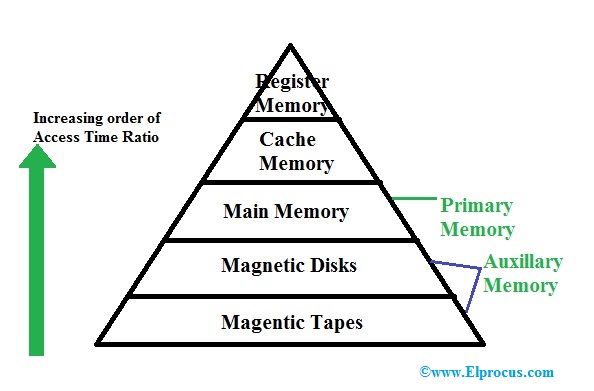
Memory hierarchy is a structure that organizes different types of memory in a computer system according to their speed, cost, and size. The goal is to balance the trade-offs between these factors to optimize overall system performance. Here’s a breakdown of the memory hierarchy, from the fastest and smallest to the slowest and largest:

1. Registers

Definition: Small, high-speed storage locations within the CPU used to hold data, instructions, and addresses temporarily during processing. They are the fastest form of memory, directly accessible by the CPU, and are used for immediate data needs.

• Characteristics:
  • Location: Part of the CPU, built directly into the processor.
  • Speed: The fastest.
  • Size: Typically very small, from a few bytes to a few kilobytes.
  • Purpose: Store temporary data such as operands for arithmetic operations, intermediate results, and instructions during execution.

---

2. Cache Memory

Definition: Fast, small-sized memory located between the CPU and main memory that stores frequently accessed data and instructions to speed up processing. It is divided into levels (L1, L2, and L3), with L1 being the smallest and fastest, and L3 being the largest and slower compared to L1 and L2.

• Characteristics:
  • Levels:
    • L1 Cache: Closest to the CPU core, extremely fast, with small capacity (32KB to 64KB per core).
    • L2 Cache: Larger than L1, slower but still faster than main memory (256KB to 1MB per core).
    • L3 Cache: Shared among multiple cores, larger (2MB to 12MB or more), slower than L1 and L2.
  • Speed: Faster than RAM and secondary storage; decreases from L1 to L3.
  • Size: L1 is the smallest, L2 is larger, and L3 is the largest.
  • Purpose: Reduces average data access time by storing frequently accessed data and instructions.

---

3. Main Memory (RAM)

Definition: Volatile memory used to store data and programs that are currently being used by the CPU. It provides a working space for active processes, offering larger capacity than cache memory but slower access speeds.

• Characteristics:
  • Type: Primarily DRAM (Dynamic RAM), slower than SRAM but more cost-effective.
  • Speed: Slower than cache memory but faster than secondary storage.
  • Size: Typically ranges from 4GB to 64GB or more.
  • Purpose: Holds data and programs that are currently in use or will be used soon.

---

4. Secondary Storage

Definition: Non-volatile storage such as hard drives and solid-state drives used to store data and applications not currently in use but needed for long-term retention. It is larger and slower compared to main memory but more cost-effective for extensive storage needs.

• Characteristics:
  • Types:
    • HDDs (Hard Disk Drives): Use spinning magnetic disks; slower but cost-effective with large capacities.
    • SSDs (Solid State Drives): Use flash memory; faster and more reliable but typically more expensive per gigabyte.
  • Speed: Slower compared to RAM but faster than tertiary storage.
  • Size: Larger, ranging from hundreds of gigabytes to several terabytes.
  • Purpose: Store data and applications not currently in use but needed long-term.

---

5. Tertiary and Off-line Storage

Definition: Long-term storage solutions like optical discs, magnetic tapes, and cloud storage used for backup, archival, and infrequent access. They provide large storage capacities and are used for data preservation and recovery, though they are the slowest among memory types.

• Characteristics:
  • Types:
    • Optical Discs (CDs/DVDs): Use laser technology; useful for archival but slow.
    • Magnetic Tapes: High capacity but very slow access times; used for large-scale backups.
    • Cloud Storage: Internet-based; offers scalability and remote access.
  • Speed: Slowest among all memory types.
  • Size: Can be very large, suitable for extensive data backups and archives.
  • Purpose: Primarily used for long-term storage, backup, and archival where speed is less critical.

Magnetic tape

Definition: Magnetic tape is a type of data storage medium that uses a thin, magnetizable coating on a strip of plastic film. Data is recorded in a sequential manner, and the tape is wound onto spools or reels. It is used primarily for long-term storage, backups, and archiving.

Characteristics:

• Speed: Relatively slow compared to other storage types. Accessing data requires sequential reading or writing, which can be time-consuming.
• Size: Very large capacity, suitable for storing vast amounts of data. Tapes can hold several terabytes of data.
• Cost: Generally low cost per gigabyte, making it cost-effective for large-scale data storage.
• Durability: Magnetic tapes are durable and can last for decades if stored properly, but they are susceptible to physical damage and magnetic interference.
• Purpose: Used for backup and archival purposes due to its high capacity and low cost. It is ideal for storing large volumes of data that do not require frequent access.

Details:

• Data Storage: Data is recorded on magnetic tape in a linear fashion, and to access data, the tape must be wound to the appropriate position. This sequential access method makes it less suitable for applications requiring random access to data.
• Types: Tapes come in various formats, such as LTO (Linear Tape-Open), DLT (Digital Linear Tape), and others, each with specific capacities and performance characteristics.
• Usage: Commonly used in data centers, libraries, and large enterprises for long-term storage solutions, especially where high capacity and low cost are more critical than speed.

1. Registers Registers are small, high-speed memory units within the CPU. They store the most frequently used data and instructions, providing the fastest access times with a typical storage capacity of 16 to 64 bits.
2. Cache Memory Cache memory is a high-speed memory unit located near the CPU. It stores recently accessed data and instructions from main memory, reducing the time required to retrieve frequently used information.
3. Main Memory Main memory, or RAM (Random Access Memory), serves as the primary memory in a computer system. It offers larger storage capacity than cache memory but operates at slower speeds. Main memory holds data and instructions currently in use by the CPU.Types of Main Memory:
   • Static RAM (SRAM): Stores binary information using flip-flops, maintaining data as long as power is supplied. It has faster access times and is used for cache memory.
   • Dynamic RAM (DRAM): Stores binary information as electrical charges in capacitors. It requires periodic refreshing to maintain data, but it can fit more memory cells per unit area compared to SRAM.
4. Secondary Storage Secondary storage, such as hard disk drives (HDDs) and solid-state drives (SSDs), is non-volatile and provides a larger storage capacity than main memory. It holds data and instructions not currently in use by the CPU. Secondary storage has slower access times and is generally less expensive.
5. Magnetic Disk Magnetic disks are circular plates made from metal, plastic, or magnetized materials. They are commonly used for high-speed data access in computers.
6. Magnetic Tape Magnetic tape is a storage medium coated with a magnetic material on a plastic film. It is typically used for data backup. Access times for magnetic tape are slower compared to other storage methods, requiring more time to retrieve data.

Characteristics of Memory Hierarchy:

• Capacity: Refers to the total amount of information a memory can store. Capacity increases as you move from the top to the bottom of the hierarchy.
• Access Time: The time between requesting data and its availability. Access time increases as you move down the hierarchy.
• Performance: Without a memory hierarchy, the speed gap between CPU registers and main memory leads to decreased system performance. Memory hierarchy improves performance by reducing the distance data must travel within the hierarchy.
• Cost Per Bit: The cost per bit increases as you move up the hierarchy, making internal memory more expensive than external storage.

Advantages of Memory Hierarchy:

• Reduces data access delays and improves memory management.
• Distributes data across the system more effectively.
• Saves cost and time for consumers.

Address Binding refers to the process of mapping logical addresses (or virtual addresses) to physical addresses in memory. It essentially allocates a physical memory region to a logical pointer, allowing programs to access memory locations accurately. This article explores address binding, its types, and their implications with an example.

What is Address Binding?

Address binding is the mapping of data and computer instructions to actual memory locations. In computer memory management, both logical and physical addresses are used. The operating system (OS) handles this mapping on behalf of programs requiring memory access.

Example:

Consider a program P1 with instructions I1, I2, I3, and I4. Suppose their logical addresses are 10, 20, 30, and 40, respectively:

• Program P1
  • I1 –> 10
  • I2 –> 20
  • I3 –> 30
  • I4 –> 40
• Program Counter: 10, 20, 30, 40

Why Do We Need Address Binding?

1. Memory Management: Address binding is crucial for effective memory management within a machine.
2. Symbol Resolution: It resolves symbolic references in a program to real memory addresses, enabling the linker/loader to correctly attach program modules, libraries, or functions.
3. Code Relocation: Address binding allows code to be relocated, enabling executable applications to be loaded into memory at different addresses each time they run.
4. Dynamic Memory Allocation: It supports dynamic memory allocation, allowing programs to request and release memory at runtime. Functions such as malloc() and free() in programming languages exemplify this capability.

Types of Address Binding

Address binding is categorized into three types:

1. Compile-Time Address Binding
2. Load-Time Address Binding
3. Execution-Time or Dynamic Address Binding

1. Compile-Time Address Binding

When address binding is performed by the compiler, it is known as compile-time binding (or static binding). During the compilation stage, symbolic addresses are linked with physical memory addresses. These addresses are fixed before the program runs, making compile-time binding straightforward and efficient. However, it lacks flexibility since the addresses cannot be adjusted during runtime. Compile-time binding is used for functions and global variables with fixed memory locations.

2. Load-Time Address Binding

Performed by the OS memory manager (i.e., the loader) after the program is loaded into memory. Load-time binding delays the address binding process until the program is ready for execution. The linker and loader assign memory addresses to variables and functions based on the memory capacity and needs. External references are resolved by the linker, replacing symbolic addresses with actual physical addresses. Load-time binding offers more flexibility than compile-time binding, as it allows addresses to adapt to runtime conditions, enabling dynamic libraries and adjustments to available memory.

3. Execution-Time or Dynamic Address Binding

This type of binding occurs during program execution. The addresses can change dynamically as the program runs. Runtime binding (or dynamic binding) allows memory addresses to be allocated and deallocated as needed, providing high flexibility. It is often used in dynamic and object-oriented programming languages where memory layout can change during execution. Runtime binding enables late binding of functions, polymorphism, and dynamic memory allocation, enhancing program adaptability.

Example of Address Binding

Scenario:

Consider a simple program Program X that performs arithmetic operations. The program contains a few variables and functions, and we will explore how address binding maps these to physical memory addresses.

Program X:

1. Variables and Functions:
   • Variable A with a logical address of 100
   • Variable B with a logical address of 200
   • Function Add() with a logical address of 300
   • Function Subtract() with a logical address of 400
2. Logical Addresses:
   • Variable A –> 100
   • Variable B –> 200
   • Function Add() –> 300
   • Function Subtract() –> 400
3. Program Counter: Points to logical addresses as the program executes.

Compile-Time Address Binding

When Program X is compiled, the compiler assigns physical addresses to the logical addresses. Suppose the physical memory available has the following base addresses:

• Variable A is mapped to physical address 5000
• Variable B is mapped to physical address 6000
• Function Add() is mapped to physical address 7000
• Function Subtract() is mapped to physical address 8000

Compile-Time Binding Result:

• Variable A –> 5000
• Variable B –> 6000
• Function Add() –> 7000
• Function Subtract() –> 8000

These mappings are fixed, and the program will always use these physical addresses during execution.

Load-Time Address Binding

When Program X is loaded into memory, the OS assigns physical addresses based on the current memory state. Suppose the program is loaded into a memory region starting at address 20000. The loader might adjust the addresses as follows:

• Variable A –> 20000 (base address) + 100 (offset) = 20100
• Variable B –> 20000 + 200 = 20200
• Function Add() –> 20000 + 300 = 20300
• Function Subtract() –> 20000 + 400 = 20400

Load-Time Binding Result:

• Variable A –> 20100
• Variable B –> 20200
• Function Add() –> 20300
• Function Subtract() –> 20400

Here, the actual physical addresses are assigned based on where the program is loaded in memory, allowing for greater flexibility compared to compile-time binding.

Execution-Time or Dynamic Address Binding

During execution, the addresses can change dynamically based on the program’s needs and memory allocation. Suppose Program X uses dynamic memory allocation to manage additional data. If Variable A is reallocated to a new memory segment, the address might be updated as follows:

• Variable A is dynamically moved to physical address 25000.
• Variable B remains at 20200.
• Function Add() remains at 20300.
• Function Subtract() remains at 20400.

Execution-Time Binding Result:

• Variable A –> 25000
• Variable B –> 20200
• Function Add() –> 20300
• Function Subtract() –> 20400

This dynamic adjustment allows for efficient memory use and supports features such as runtime polymorphism and dynamic memory allocation.

---

This example illustrates how address binding adapts at different stages: compile-time, load-time, and execution-time, demonstrating how logical addresses are mapped to physical memory addresses in each scenario.

Note: Most modern operating systems, such as Windows, Linux, and Unix, implement dynamic loading, dynamic linking, and dynamic address binding.

Conclusion

Address binding is essential for bridging the gap between physical memory addresses and the symbolic addresses used by programs. It facilitates effective memory management and smooth communication between hardware and software. The three primary forms of address binding—compile-time, load-time, and execution-time—each serve different program needs and runtime scenarios, offering various benefits and trade-offs.

Overlays

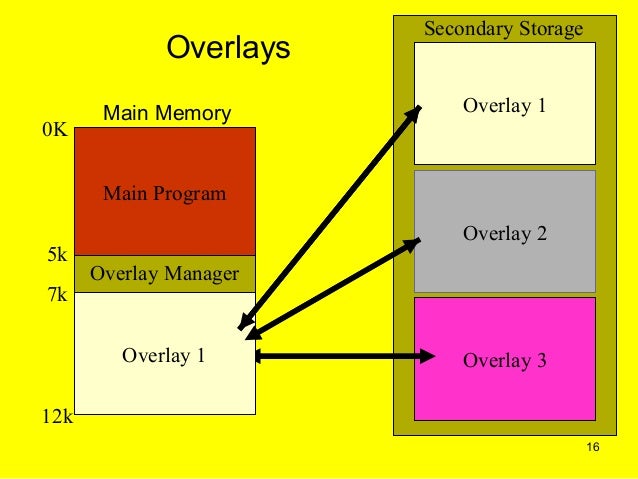
Definition: Overlays are a memory management technique used to allow a program to execute in environments where the total amount of memory is insufficient to hold the entire program and its data simultaneously. This technique involves loading and unloading different parts of a program or data into a fixed memory area as needed during execution.

Characteristics:

• Segmented Loading: Programs are divided into smaller segments or modules, known as overlays, which are loaded into a specific area of memory one at a time.
• Manual Management: The operating system or the programmer is responsible for managing which overlay is in memory at any given time.
• Efficient Use of Memory: Allows a program to handle large tasks or data structures without requiring sufficient memory to hold the entire program and all data simultaneously.

How Overlays Work:

1. Division into Overlays: The program is divided into smaller segments, each called an overlay. Each overlay contains a portion of the program or data that can be executed or used independently.
2. Loading Overlays: At runtime, only the necessary overlay is loaded into memory. The rest of the program remains on secondary storage, such as a hard disk or other storage media.
3. Switching Overlays: When a different part of the program or data is needed, the current overlay is swapped out of memory, and the new overlay is loaded in its place.
4. Overlay Management: The program or operating system tracks which overlays are loaded and manages the loading and unloading process.

Advantages:

• Memory Efficiency: Enables the execution of programs that are too large to fit entirely in memory by only loading parts of the program as needed.
• Cost-Effective: Reduces the need for large amounts of physical memory, which can be beneficial in systems with limited resources.
• Flexibility: Allows large applications to be run on systems with limited memory by managing the program’s footprint dynamically.

Disadvantages:

• Complexity: Requires careful management of overlays and can add complexity to both program design and execution.
• Performance Overhead: Frequent loading and unloading of overlays can lead to performance overhead due to disk I/O operations and context switching.
• Development Effort: The programmer must design the program with overlays in mind, which can increase development time and effort.

Applications:

• Early Computing Systems: Overlays were commonly used in early computing systems where physical memory was limited.
• Embedded Systems: Used in embedded systems with limited memory to manage large software applications.
• Specialized Software: Sometimes used in specialized applications where the memory footprint is managed carefully to optimize performance and resource usage.

Real-Life Example: Managing Tasks in a Shared Workspace

Scenario:

Imagine you have a large, multifunctional desk that can be used for various tasks—writing reports, drawing, and crafting. However, the desk is limited in space, and you can only work on one task at a time. To manage this, you use a set of overlays (such as trays or document holders) to keep your workspace organized and ensure you have the right materials available for each task without cluttering your desk.

How Overlays Work:

1. Initial Setup:
   • Task 1 (Writing Reports): You place a report folder, pens, and notepads on the desk. This is your current overlay.
   • Task 2 (Drawing): You have a separate set of materials—sketch pads, colored pencils, and erasers—which you keep in a drawer or a separate section.
2. Switching Tasks:
   • When you need to switch from writing reports to drawing, you clear the desk of report materials and replace them with drawing materials from the drawer.
   • This process of clearing and replacing materials is similar to how overlays work in computing. Only one set of data or instructions is loaded into the main memory (workspace) at a time, while other sets are stored elsewhere (drawer or separate section).

How This Relates to Computing:

• Memory Management: Just like you manage your workspace with different overlays to handle various tasks, a computer uses overlays to manage memory. It loads only the parts of a program or data that are currently needed into main memory.
• Overlay Management: In computing, an overlay system loads a portion of a program into memory (similar to putting the materials on the desk) and swaps it out with other parts as needed. This ensures that the limited memory is used efficiently.

Example in Computing:

In computing, an overlay might be used when a program is too large to fit into memory all at once. The system loads a part of the program (overlay) into memory to execute it, then swaps it out with another part when needed. For example, a large game might load the main game engine into memory and, as players progress to different levels, swap in overlays for new levels or additional assets.

In summary, just as you manage and switch between different tasks on your desk using overlays to maximize workspace efficiency, computers use overlays to manage memory and efficiently execute large programs.

Swapping

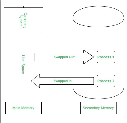
Definition: Swapping is a memory management technique used to handle situations where a computer system’s physical memory (RAM) is insufficient to accommodate all active processes. It involves moving entire processes or parts of processes between RAM and secondary storage (such as a hard disk or SSD) to free up memory for other processes.

How Swapping Works:

1. Process Selection: When the system needs to allocate memory for a new process but no free memory is available, it selects one or more processes currently in memory to be swapped out. This selection is typically based on criteria such as process priority or usage patterns.
2. Swapping Out: The selected processes are saved (swapped out) from RAM to a designated area on secondary storage, known as the swap space or swap file. This frees up physical memory for the new process.
3. Swapping In: When a process that was swapped out is needed again, it is loaded (swapped in) from secondary storage back into RAM, replacing one or more processes currently in memory.
4. Execution: The process now resides in RAM and can resume execution from where it was paused before being swapped out.

Characteristics:

• Swap Space: The area on secondary storage used to hold swapped-out processes. It can be a dedicated partition, a swap file, or a combination of both.
• Swapping Granularity: Swapping can be done at the level of entire processes or individual pages (in systems with paging).

Advantages:

• Increased System Utilization: Allows more processes to be executed simultaneously by using secondary storage as an extension of RAM.
• Flexibility: Provides the ability to handle larger workloads or more processes than the physical memory alone would allow.

Disadvantages:

• Performance Overhead: Swapping involves significant I/O operations, which can lead to slower performance compared to when all processes are kept in RAM. The latency of accessing data from secondary storage is much higher than from RAM.
• Increased Complexity: Managing swapping can add complexity to the operating system’s memory management, including maintaining the state of processes and handling swap space efficiently.
• Thrashing: If the system is constantly swapping processes in and out of memory due to insufficient RAM, it can lead to thrashing, where the system spends more time swapping than executing processes, significantly degrading performance.

Applications:

• Multi-tasking Systems: Swapping is commonly used in multi-tasking operating systems where multiple processes or applications need to be managed concurrently, even when physical memory is limited.
• Virtual Memory Systems: In systems with virtual memory, swapping works in conjunction with paging to manage memory more effectively by swapping pages of memory in and out of RAM.

Real-Life Example: Managing a Large Number of Books

Scenario:

Imagine you have a small bookshelf (representing the main memory) that can only hold a limited number of books. You have a large collection of books (representing processes or programs) that you need to manage. You can’t fit all of them on the shelf at once, so you need a strategy to manage them efficiently.

How Swapping Works:

1. Initial Setup:
   • You place a few books on the shelf that you are currently reading or need frequently. These are the “active” books.
   • The rest of the books are stored in a storage area, such as a box or a closet (representing the disk or swap space).
2. Switching Books:
   • When you finish reading some books or need to access others, you remove the books you no longer need from the shelf and replace them with books from the storage area.
   • This process of moving books in and out of the storage area is similar to how swapping works in a computer.

How This Relates to Computing:

• Memory Management: Just like you manage your bookshelf space by swapping books in and out, a computer manages memory by swapping processes or data between RAM and a disk storage area.
• Swapping Process:
  • When a process needs more memory than is available, or when the operating system decides that it’s more efficient to free up memory for other tasks, the system saves the current process’s state to the disk (swap space).
  • It then loads the required process or data into RAM, allowing the system to continue working efficiently without running out of memory.

Benefits:

• Efficiency: Swapping allows the system to handle more processes than can fit into RAM simultaneously, optimizing the use of available memory.
• Flexibility: By moving processes in and out of memory, the system can manage multiple applications and tasks, improving overall performance and responsiveness.

Example in Computing:

Consider a scenario where you’re running several applications on your computer, and the total memory needed exceeds the available RAM. Here’s how swapping would work:

1. Active Process: Your word processor and web browser are currently in use, and their data is in RAM.
2. Memory Demand: You open a large image editing application that requires more memory than available.
3. Swapping Action: The operating system moves some of the less frequently used data from RAM (e.g., parts of the word processor or browser data) to the disk swap space to free up RAM.
4. Loading New Process: The image editing application is then loaded into the now available RAM.
5. Swapping Back: If you switch back to the word processor or browser, the system will swap out the image editing data and bring back the necessary data from disk.

Swapping helps to ensure that the computer can handle multiple processes by efficiently managing memory and disk space, similar to how you manage limited shelf space by rotating books in and out.

Single Partition Allocation

Definition: Single partition allocation is a memory management technique where the entire physical memory is allocated to a single process or job at a time. This approach means that only one process can occupy the memory space at any given moment, and the process has exclusive access to the entire memory.

Characteristics:

1. Exclusive Allocation:
   • The entire memory space is dedicated to a single process or job.
   • No other process can use the memory until the current process completes and releases the memory.
2. Simple Implementation:
   • This method is straightforward to implement, as it does not require complex memory management algorithms.
3. Fixed Allocation:
   • The allocation of memory is fixed for the duration of the process. Once a process starts, it cannot be moved or resized until it finishes.

Advantages:

1. Simplicity:
   • The approach is simple to implement and manage, as it avoids the complexities of partitioning and dynamic memory allocation.
2. No Fragmentation:
   • Since only one process uses the memory at a time, there is no issue of fragmentation (both internal and external) within the memory space.
3. Predictable Performance:
   • The entire memory is dedicated to the process, so the process does not experience delays or performance issues related to other processes.

Disadvantages:

1. Inefficiency:
   • This method can lead to inefficient use of memory if the allocated process does not fully utilize the available memory.
   • The entire memory is reserved for one process, which can lead to underutilization if the process’s memory requirements are lower than the allocated memory.
2. Poor Multitasking:
   • Single partition allocation is not conducive to multitasking, as it only supports one process at a time. Modern operating systems need to support multiple processes simultaneously.
3. No Memory Sharing:
   • There is no mechanism for sharing memory between processes, which limits the ability to handle multiple concurrent tasks.

Applications:

1. Early Computer Systems:
   • This method was commonly used in early computer systems where hardware resources were limited and processes were not designed for multitasking.
2. Simple Systems:
   • Suitable for simple or dedicated systems where only one process or job needs to run at a time, such as some embedded systems or single-use applications.

Real-Life Example: Managing a Single Large Desk

Scenario:

Imagine you have a large desk in an office that is used for various tasks. However, this desk can only accommodate one task at a time. Whenever you start a new task, you must clear the desk of all materials from the previous task before you can begin the new one.

How Single Partition Allocation Works:

1. Initial Setup:
   • You start with a clear desk (memory).
   • You place materials for Task 1 on the desk.
2. Working on Task 1:
   • All your work for Task 1 is done using the desk space.
3. Switching Tasks:
   • Once Task 1 is completed, you clear the desk of Task 1’s materials.
   • You then set up the desk with materials for Task 2.
4. Starting Task 2:
   • The desk is now fully dedicated to Task 2, and Task 1’s materials are not visible or accessible.

How This Relates to Computing:

• Exclusive Allocation: Similar to the desk, the memory is exclusively allocated to one process at a time.
• Clearance Required: Just as you need to clear the desk before starting a new task, the memory needs to be cleared before loading a new process.
• Simple Management: Managing a single partition is straightforward because you only need to handle one process at a time.

Example in Computing:

Consider a computer system with 8 GB of RAM using single partition allocation. When you run a large application that requires 4 GB of memory, the entire 8 GB RAM is dedicated to that application, even though it only uses 4 GB. During this time, no other applications can use the remaining 4 GB of RAM.
In summary, single partition allocation is a simple memory management technique where the entire memory is allocated to a single process. While it simplifies management and avoids fragmentation, it can lead to inefficient memory usage and does not support concurrent processes.

Conclusion:

Single partition allocation is a straightforward memory management technique that allocates the entire memory space to a single process or job. While it is simple and avoids fragmentation issues, it is inefficient for systems requiring multitasking and can lead to underutilization of memory resources. Modern operating systems typically use more advanced memory management techniques, such as partitioning, paging, or segmentation, to support multiple concurrent processes and optimize memory usage.

Multiple Partitioned allocation

Multiple Partition Allocation

Definition: Multiple partition allocation is a memory management technique where the physical memory is divided into several fixed or variable-sized partitions. Each partition can be allocated to a different process or job simultaneously. This approach allows multiple processes to be executed concurrently by utilizing different segments of memory.

Characteristics:

1. Partitioning Memory:
   • Fixed Partitioning: The memory is divided into a set number of fixed-size partitions. Each partition is allocated to a single process. The size of the partitions is determined at system setup.
   • Variable Partitioning: The memory is divided into partitions of varying sizes based on the needs of the processes. Partitions are created dynamically as needed, and their sizes can vary.
2. Multiple Processes:
   • Multiple processes can reside in memory at the same time, each occupying a separate partition. This facilitates multitasking and improved resource utilization.
3. Allocation Mechanism:
   • Processes are allocated to available partitions based on their size and the size of the partitions. In fixed partitioning, processes fit into predefined partitions, while in variable partitioning, partitions are created dynamically to fit the processes.

Advantages:

1. Improved Utilization:
   • Fixed Partitioning: Although fixed partitions may lead to some internal fragmentation (unused space within partitions), it allows for straightforward memory management.
   • Variable Partitioning: Reduces internal fragmentation by allocating partitions that fit the size of the processes more closely.
2. Multitasking:
   • Supports concurrent execution of multiple processes, making better use of available memory resources compared to single partition allocation.
3. Flexibility:
   • Fixed Partitioning: Simple to implement and manage, as partitions do not change size.
   • Variable Partitioning: More flexible in terms of adapting to the memory needs of different processes.

Disadvantages:

1. Fragmentation:
   • Fixed Partitioning: May lead to internal fragmentation if processes are smaller than the fixed partition size.
   • Variable Partitioning: Can lead to external fragmentation, where free memory is split into small, non-contiguous blocks, making it difficult to allocate memory for larger processes.
2. Complexity:
   • Variable Partitioning: Requires more complex management of partitions and memory allocation, including tracking free and occupied memory blocks.
3. Overhead:
   • Managing multiple partitions can introduce overhead related to tracking and managing the different partitions and their allocations.

Applications:

1. Early Operating Systems:
   • Used in early operating systems and mainframes where fixed partitioning provided a simple method for multitasking.
2. Modern Systems:
   • Variable partitioning techniques are used in modern systems with more advanced memory management features, such as dynamic memory allocation and garbage collection.

Real-Life Example: Office Cubicles

Scenario:

Imagine an office with several cubicles (partitions) of varying sizes. Each cubicle can be occupied by one employee (process) at a time. The office can accommodate multiple employees concurrently, each working in their designated cubicle.

How Multiple Partitioned Allocation Works:

1. Initial Setup:
   • The office has several cubicles of different sizes, such as small, medium, and large.
   • Each cubicle is empty and available for use.
2. Employee Assignment:
   • When a new employee joins the office, they are assigned a cubicle based on their needs. For example, a large project team might require a large cubicle, while a single worker might need only a small cubicle.
3. Concurrent Work:
   • Multiple employees can work concurrently in their assigned cubicles. Each cubicle is occupied by one employee, and no cubicle is shared among multiple employees.
4. Cubicle Management:
   • When an employee leaves or finishes their task, the cubicle is cleared and becomes available for another employee.

How This Relates to Computing:

• Multiple Processes: Just like multiple employees can work concurrently in different cubicles, multiple processes can be loaded into different memory partitions at the same time.
• Efficient Utilization: Memory is utilized more efficiently because it is divided into partitions that can be allocated to processes of varying sizes.
• Partition Management: The operating system manages the allocation and deallocation of memory partitions based on process requirements.

Types of Multiple Partition Allocation:

1. Fixed Partition Allocation:
   • Memory is divided into a set number of partitions of fixed size.
   • Each partition can hold only one process.
   • Advantages: Simple to implement, avoids external fragmentation.
   • Disadvantages: May lead to internal fragmentation if processes are smaller than the partition size.
2. Variable Partition Allocation:
   • Memory is divided into partitions of variable sizes, allocated dynamically based on process needs.
   • Advantages: More flexible and efficient use of memory, reduces internal fragmentation.
   • Disadvantages: Can lead to external fragmentation, where free memory is available but not contiguous.

Example in Computing:

Consider a system with 16 GB of RAM using variable partition allocation:

1. Partition Allocation:
   • A 2 GB process is allocated a 2 GB partition.
   • A 4 GB process is allocated a 4 GB partition.
   • A 1 GB process is allocated a 1 GB partition.
2. Concurrent Processes:
   • All three processes are loaded and running concurrently, each in its allocated partition.
3. Fragmentation:
   • Over time, as processes are loaded and removed, the memory might become fragmented with small gaps of free memory.

In summary, multiple partitioned allocation improves memory utilization by allowing multiple processes to run concurrently in different partitions. It can be implemented with fixed or variable partition sizes, each with its own advantages and trade-offs in terms of fragmentation and memory management complexity.

Conclusion:

Multiple partition allocation is an effective technique for managing memory in systems that need to run multiple processes concurrently. Fixed partitioning offers simplicity and straightforward management, while variable partitioning provides flexibility and better memory utilization by adapting partition sizes to process requirements. However, both approaches have their challenges, including fragmentation and complexity, which modern systems address using advanced memory management techniques such as paging and segmentation.

Definition: Fragmentation refers to the phenomenon where free memory is broken into small, non-contiguous blocks, which can lead to inefficient utilization of memory and difficulties in allocating large contiguous memory spaces. Fragmentation can occur in both main memory (RAM) and secondary storage, such as hard drives or SSDs.

Types of Fragmentation:

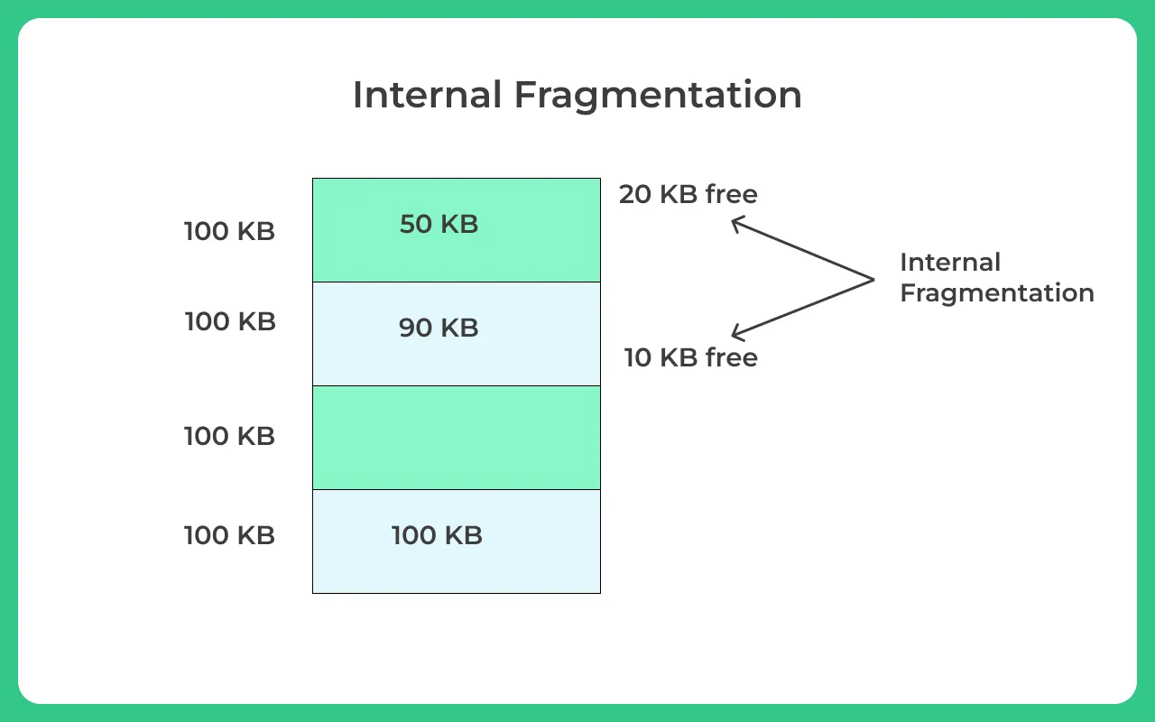
definition: Internal fragmentation occurs when allocated memory may be larger than the required amount for a process, resulting in wasted space within the allocated partition or block.

Example: If a fixed-size partition of 256 MB is allocated to a process that only requires 100 MB, the remaining 156 MB within that partition is wasted and cannot be used by other processes.

Cause: Typically caused by fixed partitioning or allocation strategies where memory blocks or partitions are larger than what is needed by the processes.

Allocation Strategies:

1. Best Fit
   • Definition: Allocates the smallest block of memory that fits the process’s request. It tries to minimize wasted space by choosing the closest match.
   • Impact on Internal Fragmentation: Minimizes internal fragmentation by choosing the smallest adequate block. However, it can lead to external fragmentation, where many small unusable blocks remain.
   • Real-Life Example:Suppose you have three bins of different sizes: 10 liters, 20 liters, and 30 liters. You need a bin for 8 liters of liquid. The best fit strategy would choose the 10-liter bin because it fits the requirement best while minimizing unused space. The 2 liters left in the 10-liter bin represent internal fragmentation.
2. First Fit
   • Definition: Allocates the first block of memory that is large enough to satisfy the request, scanning memory from the start.
   • Impact on Internal Fragmentation: Can result in more internal fragmentation than the best fit, as it might choose a larger block than necessary. This approach may lead to inefficient use of space if the block chosen is much larger than needed.
   • Real-Life Example:Imagine a series of boxes of different sizes on a shelf: 5 liters, 15 liters, and 25 liters. You need a box for 8 liters of liquid. Using the first fit strategy, you would pick the 15-liter box because it’s the first box that fits the requirement. The 7 liters left in the 15-liter box represent internal fragmentation.
3. Worst Fit
   • Definition: Allocates the largest available block of memory, aiming to leave the largest possible remaining free blocks.
   • Impact on Internal Fragmentation: Can increase internal fragmentation because it allocates a large block of memory even if a smaller block would suffice. This strategy aims to prevent too many small unusable fragments but can leave large amounts of unused space in each allocated block.
   • Real-Life Example:Suppose you have three bins of sizes: 15 liters, 25 liters, and 35 liters. You need a bin for 8 liters of liquid. The worst fit strategy would choose the 35-liter bin to ensure that the largest remaining space is left. This results in 27 liters of internal fragmentation in the 35-liter bin.

1. External Fragmentation:

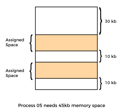
Let’s take the example of external fragmentation. In the above diagram, you can see that there is sufficient space (50 KB) to run a process (05) (need 45KB), but the memory is not contiguous. You can use compaction, paging, and segmentation to use the free space to execute a process.

Effects of Fragmentation:

• Reduced Efficiency: Fragmentation can lead to inefficient use of memory, with significant portions of memory remaining unused.
• Increased Overhead: More time and effort are required to manage fragmented memory and find suitable blocks for allocation.
• Performance Degradation: Systems may experience slower performance due to the overhead of managing fragmented memory and the potential for increased swapping or paging.

Solutions to Fragmentation:

1. Compaction:
   • Definition: Compaction involves reorganizing memory to combine fragmented free blocks into contiguous spaces. This process moves processes or data to create larger contiguous blocks of free memory.
   • Use: Effective in addressing external fragmentation by reducing the number of small, scattered free blocks.
2. Paging:
   • Definition: Paging is a memory management technique that divides memory into fixed-size blocks called pages. Processes are also divided into pages, and these pages can be loaded into any available memory location, reducing fragmentation.
   • Use: Helps manage both internal and external fragmentation by using fixed-size blocks, which simplifies memory allocation and reduces fragmentation.
3. Segmentation:
   • Definition: Segmentation divides memory into variable-sized segments based on the logical divisions of processes, such as code, data, and stack segments. Each segment can be allocated separately.
   • Use: Helps manage memory more flexibly and can reduce fragmentation compared to fixed-sized partitions.
4. Dynamic Memory Allocation Algorithms:
   • Best Fit: Allocates the smallest free block that fits the process size, reducing wasted space but potentially increasing fragmentation.
   • First Fit: Allocates the first sufficiently large block, which can lead to fragmentation over time but is generally faster.
   • Worst Fit: Allocates the largest free block, aiming to leave larger remaining blocks, though this method can also lead to fragmentation.

Example Scenario:

Consider a computer system using variable-sized memory allocation. Over time, as processes are loaded and unloaded, free memory becomes fragmented into small, non-contiguous blocks. When a new process that requires a large contiguous block of memory needs to be allocated, it may not fit into the scattered free blocks even though the total free memory is sufficient. This situation exemplifies external fragmentation.

Addressing Fragmentation:

To manage fragmentation, the system might periodically perform compaction to combine free memory blocks into larger contiguous areas or use paging and segmentation to better handle memory allocation. These techniques help maintain efficient memory utilization and minimize the negative effects of fragmentation.

Conclusion:

Fragmentation is a key challenge in memory management that affects both internal and external memory usage. Internal fragmentation results from inefficient use of allocated memory within fixed-size partitions, while external fragmentation occurs when free memory is scattered in non-contiguous blocks. Various techniques, such as compaction, paging, and segmentation, are employed to manage and mitigate the effects of fragmentation, ensuring more efficient use of memory resources.

Paging Concept

Definition: Paging is a memory management technique that divides the computer’s physical memory into fixed-size blocks called “pages.” Similarly, processes are divided into blocks of the same size, known as “page frames” or simply “pages.” Paging allows the system to manage memory more efficiently and reduces the issues of fragmentation.

How Paging Works:

1. Memory Division:
   • Page Size: Memory is divided into fixed-size blocks called pages. Common page sizes are 4 KB, 8 KB, or 16 KB.
   • Page Frames: The physical memory is divided into page frames of the same size as the pages used by processes.
2. Process Division:
   • Logical Pages: A process is divided into logical pages of the same size as the physical pages.
   • Page Table: Each process has a page table that maps logical pages to physical page frames. The page table keeps track of where each page is stored in physical memory.
3. Address Translation:
   • Logical Address: Consists of a page number and an offset within the page.
   • Physical Address: Determined by translating the logical page number using the page table to find the corresponding physical page frame, then combining it with the offset.

Paging Mechanism:

1. Loading Pages:
   • Page Request: When a process needs to access data, the system checks if the required page is in physical memory (RAM).
   • Page Fault: If the page is not in RAM (a page fault occurs), the operating system retrieves it from secondary storage (e.g., hard drive) and loads it into a free page frame.
2. Page Replacement:
   • When Memory is Full: If physical memory is full and a new page needs to be loaded, the system must decide which page to evict. Common page replacement algorithms include Least Recently Used (LRU), FIFO (First In, First Out), and Optimal Page Replacement.

Advantages of Paging:

1. Eliminates External Fragmentation:
   • Since memory is divided into fixed-size pages, there is no issue of external fragmentation. Free memory is always available in units of pages, making allocation more efficient.
2. Simplifies Memory Management:
   • Paging simplifies memory allocation by dealing with fixed-size blocks. It makes it easier to manage memory and load processes into any available space.
3. Supports Virtual Memory:
   • Paging is a fundamental technique for implementing virtual memory, allowing processes to use more memory than physically available by swapping pages in and out of RAM.

Disadvantages of Paging:

1. Internal Fragmentation:
   • Inside Pages: Although paging eliminates external fragmentation, it can still lead to internal fragmentation if the process does not completely fill the allocated page, resulting in wasted space within the page.
2. Overhead:
   • Page Table Management: Maintaining page tables and handling page faults adds overhead to the system. The size of the page table can be substantial, especially with large amounts of memory.
3. Performance Issues:
   • Page Faults: Frequent page faults can degrade system performance, as accessing data from secondary storage is much slower than accessing it from RAM.

Real-Life Example:

Imagine a university with a fixed number of classrooms (pages) and students (processes). Each classroom can hold a fixed number of students, and each student (process) is assigned a specific desk (page) in one of the classrooms. If a new student arrives and there’s no free desk, a student who has been sitting idle for a long time might be moved to a different classroom to make room for the new student. This ensures that classrooms are utilized efficiently, and no classroom remains partially empty while there is a need for more space.

Example

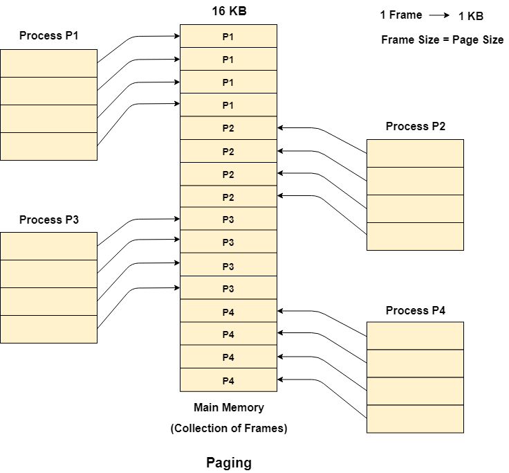
Let us consider the main memory size 16 Kb and Frame size is 1 KB therefore the main memory will be divided into the collection of 16 frames of 1 KB each.
There are 4 processes in the system that is P1, P2, P3 and P4 of 4 KB each. Each process is divided into pages of 1 KB each so that one page can be stored in one frame.
initially, all the frames are empty therefore pages of the processes will get stored in the contiguous way.
Frames, pages and the mapping between the two is shown in the image below

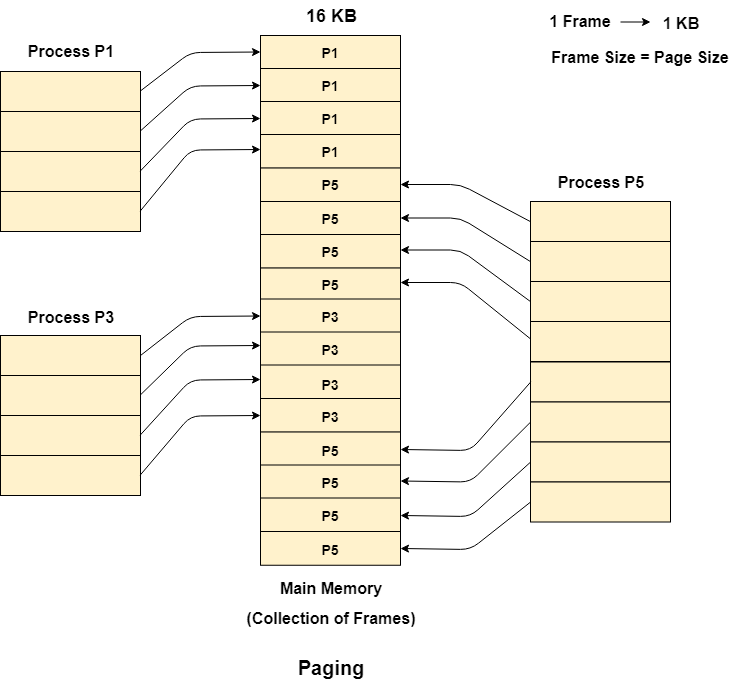
Let us consider that, P2 and P4 are moved to waiting state after some time. Now, 8 frames become empty and therefore other pages can be loaded in that empty place. The process P5 of size 8 KB (8 pages) is waiting inside the ready queue.

Given the fact that, we have 8 non contiguous frames available in the memory and paging provides the flexibility of storing the process at the different places. Therefore, we can load the pages of process P5 in the place of P2 and P4.

Paging Summary:

Paging is an effective memory management technique that divides memory and processes into fixed-size blocks, allowing for more efficient memory use and reducing fragmentation. By using page tables to map logical addresses to physical addresses, paging facilitates the implementation of virtual memory, supports multitasking, and simplifies memory allocation. However, it also introduces some overhead and potential performance issues, which are managed through various algorithms and optimizations.

Segmentation

Segmentation Concept

Definition: Segmentation is a memory management technique where the memory is divided into variable-sized segments based on the logical divisions of a program. Unlike paging, which uses fixed-size blocks, segmentation uses segments that correspond to different parts of a process such as code, data, stack, and heap.

How Segmentation Works:

1. Memory Division:
   • Segments: The logical address space of a process is divided into segments. Each segment represents a different logical unit of the process, such as:
     • Code Segment: Contains the executable code of the process.
     • Data Segment: Contains global and static variables.
     • Stack Segment: Contains stack data used for function calls and local variables.
     • Heap Segment: Used for dynamic memory allocation.
2. Segment Table:
   • Segment Table: Each process has a segment table that maintains the mapping of segment numbers to physical memory addresses.
     • Base Address: The starting address of the segment in physical memory.
     • Limit (Length): The size of the segment.
3. Address Translation:
   • Logical Address: Consists of a segment number and an offset within that segment.
   • Physical Address: Calculated by translating the segment number using the segment table to find the base address of the segment, then adding the offset to the base address.

Segmentation Mechanism:

1. Loading Segments:
   • Segment Request: When a process needs to access data, the system uses the segment number to find the segment’s base address and then calculates the physical address by adding the offset.
2. Segment Fault:
   • Segment Not Loaded: If the segment is not currently in memory (a segment fault occurs), the operating system retrieves it from secondary storage and loads it into a free segment of physical memory.
3. Protection and Sharing:
   • Protection: Segmentation allows for memory protection at the segment level, where access rights can be set for each segment (e.g., read-only or read-write).
   • Sharing: Segments can be shared between processes, such as shared libraries or code segments.

Advantages of Segmentation:

1. Logical Organization:
   • Segmentation reflects the logical structure of a program, making it easier to manage and understand memory allocation based on program units.
2. Flexibility:
   • Allows variable-sized segments, which can adapt to the needs of different program components, reducing internal fragmentation.
3. Protection and Isolation:
   • Provides protection and isolation between different segments, enhancing security and stability.

Disadvantages of Segmentation:

1. External Fragmentation:
   • Segmentation can lead to external fragmentation where free memory is scattered in non-contiguous blocks, making it difficult to allocate large segments.
2. Complexity in Management:
   • Managing variable-sized segments and their mappings can be more complex compared to fixed-size paging.

For Example:

Suppose a 16 bit address is used with 4 bits for the segment number and 12 bits for the segment offset so the maximum segment size is 4096 and the maximum number of segments that can be refereed is 16.
When a program is loaded into memory, the segmentation system tries to locate space that is large enough to hold the first segment of the process, space information is obtained from the free list maintained by memory manager. Then it tries to locate space for other segments. Once adequate space is located for all the segments, it loads them into their respective areas.

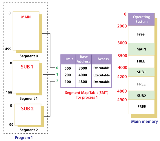
With the help of segment map tables and hardware assistance, the operating system can easily translate a logical address into physical address on execution of a program.
The Segment number is mapped to the segment table. The limit of the respective segment is compared with the offset. If the offset is less than the limit then the address is valid otherwise it throws an error as the address is invalid.
In the case of valid addresses, the base address of the segment is added to the offset to get the physical address of the actual word in the main memory.
The above figure shows how address translation is done in case of segmentation.

Segmentation with Paging

Definition: Segmentation with paging is a memory management technique that combines the concepts of segmentation and paging to leverage the advantages of both methods. This hybrid approach uses segments to reflect the logical structure of a program and then divides these segments into pages to manage memory more efficiently.

How Segmentation with Paging Works:

1. Memory Division:
   • Segments: The logical address space of a process is divided into segments, each representing a different logical unit of the program (e.g., code, data, stack, heap).
   • Pages: Each segment is further divided into fixed-size pages.
2. Segment Table:
   • Segment Table: Each process has a segment table that maps segment numbers to physical memory locations.
     • Base Address: The starting address of the segment in physical memory.
     • Limit: The size of the segment.
3. Page Table for Each Segment:
   • Segment Page Table: Each segment has its own page table that maps logical pages within the segment to physical page frames.
     • Page Table Entries: Each entry in the segment’s page table contains the base address of the page frame in physical memory.
4. Address Translation:
   • Logical Address: Consists of a segment number, a page number within the segment, and an offset within the page.
   • Physical Address: Calculated by:
     • Using the segment number to find the base address of the segment from the segment table.
     • Using the page number within the segment to find the base address of the page frame from the segment’s page table.
     • Adding the offset within the page to get the final physical address.

Segmentation with Paging Mechanism:

1. Loading Pages:
   • Segment and Page Request: When a process accesses data, the system first looks up the segment table to find the base address of the segment. Then, it uses the segment’s page table to find the base address of the page frame and calculates the physical address.
2. Segment and Page Faults:
   • Segment Fault: If the segment is not in memory, it must be loaded from secondary storage.
   • Page Fault: If the page within the segment is not in memory, it must be loaded from secondary storage into a free page frame.
3. Protection and Sharing:
   • Protection: Memory protection is managed at both the segment and page levels, providing fine-grained access control.
   • Sharing: Segments can be shared among processes, and pages within segments can be shared as well.

Advantages of Segmentation with Paging:

1. Combines Benefits:
   • Logical Organization: Segmentation provides a logical view of memory, reflecting the structure of a program.
   • Efficient Memory Use: Paging eliminates external fragmentation and makes memory management more flexible.
2. Flexibility and Protection:
   • Variable-sized Segments: Allows for efficient management of varying-sized data structures.
   • Fine-grained Protection: Enables protection and sharing at both segment and page levels.
3. Supports Virtual Memory:
   • Paging in Segments: Enhances the implementation of virtual memory by combining segment-based logical organization with the efficient paging mechanism.

Disadvantages of Segmentation with Paging:

1. Complexity:
   • Increased Overhead: Managing both segment tables and page tables increases system complexity and overhead.
2. Potential for Increased Fragmentation:
   • Internal Fragmentation: Still possible within pages if the allocated page size is larger than the required space.
   • External Fragmentation: Can occur at the segment level if memory is not efficiently managed.

Real-Life Example:

Scenario: Consider a university’s library system that manages various types of documents (e.g., textbooks, journals, research papers).

1. Segments:
   • Code Segment: Handles the cataloging system.
   • Data Segment: Stores information about each document (e.g., metadata, author).
   • Stack Segment: Manages temporary data while searching or cataloging.
   • Heap Segment: Used for dynamic additions to the library system.
2. Paging:
   • Within Each Segment: Each segment is further divided into fixed-size pages for efficient storage and retrieval of documents.
3. Address Translation:
   • Logical Address: [Segment Number] [Page Number] [Offset]
   • Segment Table Lookup: Determines the base address of the segment.
   • Page Table Lookup: Determines the base address of the page frame within the segment.
   • Physical Address Calculation: Combines the base address from the page table with the offset to locate the document’s exact location.

Visual Representation:

1. Logical Address Space:

Pages Within Each Segment:

Code Segment: [Page 0 | Page 1 | Page 2 | ...]
Data Segment: [Page 0 | Page 1 | Page 2 | ...]

Segment Table:

Segment Number	Base Address	Limit
0 (Code)	0x1000	0x2000
1 (Data)	0x3000	0x1000
2 (Stack)	0x4000	0x0800
3 (Heap)	0x4800	0x1800

Page Table for a Segment:

Page Number	Frame Number
0	2
1	5
2	1

Address Translation Example:

• Given: Logical Address = Segment 1, Page 2, Offset 0x50
• Segment Table Lookup:
  • Base Address for Segment 1: 0x3000
• Page Table Lookup for Segment 1:
  • Page Frame for Page 2: 1
• Physical Address Calculation:
  • Base Address of Page Frame 1: 0x1000
  • Physical Address: 0x1000 + 0x50 = 0x1050

Conclusion:

Segmentation with paging combines the logical organization of segmentation with the efficient memory management of paging. This hybrid approach enhances flexibility, protection, and support for virtual memory while managing complexity and potential fragmentation.

Virtual Memory

Definition: Virtual memory is a memory management technique that creates an illusion of a large, contiguous block of memory for applications, even if the physical memory (RAM) is fragmented or limited. It allows a system to use disk space as an extension of RAM, making it possible to run more applications concurrently or handle larger applications than would otherwise fit into physical memory alone.

Key Concepts:

1. Virtual Address Space:
   • Each process is given its own virtual address space, which the operating system maps to physical memory locations. This provides each process with a large, contiguous addressable space, regardless of the actual physical memory layout.
2. Paging and Segmentation:
   • Paging: Virtual memory is divided into fixed-size pages. The physical memory is divided into corresponding page frames. When a process accesses a page, the operating system maps it to a physical page frame, potentially swapping it in and out of disk storage as needed.
   • Segmentation: Virtual memory can also be divided into segments of varying sizes. Each segment can be independently mapped to physical memory. This approach provides more flexibility than paging but can be more complex to manage.
3. Page Table:
   • The page table is a data structure used by the operating system to keep track of the mapping between virtual addresses and physical addresses. It translates virtual addresses used by a process into physical addresses in RAM.
4. Page Faults:
   • When a process tries to access a page that is not currently in physical memory, a page fault occurs. The operating system must handle the page fault by loading the required page from disk into physical memory, which may involve swapping out another page to make room.
5. Swapping:
   • Swapping is the process of moving pages between physical memory and disk storage to manage memory demands. It ensures that the most frequently used pages remain in physical memory while less frequently used pages are swapped out to disk.

Real-Life Analogy:

Office Filing System:

Imagine a large office with a filing cabinet (RAM) that can only hold a limited number of folders (documents). However, the office deals with many more documents than can fit in the cabinet at one time.

1. Virtual Filing Cabinet:
   • Each employee (process) has access to their own virtual filing cabinet (virtual address space) that appears to be as large as they need, even though the actual physical cabinet is smaller.
2. Document Retrieval:
   • If an employee needs a document that is not currently in the filing cabinet, they request it from an archive (disk storage). The document is retrieved from the archive and placed into the cabinet, and possibly, another document is temporarily removed to make space.
3. Efficient Use of Space:
   • By using the archive, the office can efficiently manage a large number of documents without needing an equally large physical cabinet. This allows employees to work with more documents than would fit in the cabinet at once.

Advantages of Virtual Memory:

1. Increased Memory Capacity:
   • Virtual memory allows applications to use more memory than physically available by utilizing disk space as an extension of RAM.
2. Isolation and Protection:
   • Virtual memory provides process isolation by giving each process its own virtual address space. This prevents processes from interfering with each other’s memory.
3. Efficient Memory Use:
   • By swapping pages in and out of disk storage, the system can efficiently manage memory and prioritize active processes, improving overall system performance.
4. Simplified Memory Management:
   • Virtual memory simplifies memory management for applications by providing a uniform and contiguous address space, making programming easier and more efficient.

Disadvantages of Virtual Memory:

1. Performance Overhead:
   • Accessing data from disk is slower than accessing data from RAM. Frequent page faults and swapping can lead to performance degradation known as “thrashing,” where the system spends more time swapping pages than executing processes.
2. Disk Space Usage:
   • Virtual memory requires disk space to store swapped-out pages. If disk space is insufficient, the system may become unstable or unable to handle additional memory demands.
3. Complexity:
   • Implementing and managing virtual memory requires complex algorithms and data structures, such as page tables and swapping mechanisms, adding overhead to system operations.

Conclusion:

Virtual memory is a crucial technology in modern operating systems that enhances memory management by providing an extended, contiguous address space for applications, even with limited physical RAM. It improves system performance and multitasking capabilities but introduces challenges such as potential performance overhead and increased disk space usage. By effectively managing memory resources, virtual memory enables systems to run larger applications and handle more processes concurrently.

Demand Paging

Demand Paging is a memory management technique that delays loading pages into physical memory until they are needed by a process. This approach is a form of lazy loading, where pages are only brought into memory when a page fault occurs, meaning the program attempts to access a page that is not currently in RAM. Demand paging helps optimize memory usage and allows for more efficient execution of programs by only loading the essential portions of a program into memory.

How Demand Paging Works:

1. Initial State:
   • When a process starts, its pages are not immediately loaded into memory. Instead, they reside on the disk in a space known as the backing store or swap space.
2. Page Table Setup:
   • Each process has a page table that keeps track of the mapping between virtual pages and physical frames. Initially, the page table entries indicate that the pages are not in memory (marked as invalid or absent).
3. Page Fault Occurrence:
   • When a process tries to access a page that is not present in physical memory, a page fault is triggered. The operating system intercepts this fault to handle it.
4. Page Fault Handling:
   • Disk Access: The operating system locates the needed page in the backing store and loads it into a free frame in physical memory.
   • Page Table Update: The page table is updated to reflect the new mapping of the virtual page to the physical frame. The entry for the page is marked as valid.
   • Process Resumption: Once the page is loaded and the page table is updated, the process can resume execution from the point where it was interrupted by the page fault.
5. Page Replacement (if needed):
   • If there are no free frames available in physical memory, the operating system must use a page replacement algorithm to select a page to evict from memory to make room for the new page.

Advantages of Demand Paging:

1. Efficient Memory Use:
   • Only the necessary pages are loaded into memory, allowing the system to utilize available RAM more efficiently. This is especially beneficial for large applications or systems with limited physical memory.
2. Faster Process Startup:
   • Programs can start executing without having to load all their pages into memory, reducing initial loading times and improving system responsiveness.
3. Reduced I/O Overhead:
   • Demand paging reduces disk I/O operations by only loading pages that are actively accessed by the process, minimizing unnecessary data transfers between disk and memory.
4. Support for Overcommitment:
   • Systems can run more processes than the available physical memory can hold simultaneously by swapping pages in and out as needed. This enables better multitasking and resource utilization.

Disadvantages of Demand Paging:

1. Page Fault Overhead:
   • Frequent page faults can degrade system performance, as handling page faults involves additional overhead for disk access and memory management operations.
2. Thrashing:
   • If the system is overcommitted and processes constantly require pages that are not in memory, the system may spend more time handling page faults than executing processes. This phenomenon is known as thrashing, which severely degrades performance.
3. Latency:
   • Accessing a page not in memory introduces latency due to the time taken to load the page from disk. This can affect the performance of applications with high memory access demands.

Real-Life Analogy

Library Book Checkout:

Imagine a library with limited shelf space (physical memory). The library has a vast collection of books (process pages), but not all books can fit on the shelves at once. Here’s how demand paging works in this context:

1. Books in Storage:
   • Most books are kept in a storage room (backing store/disk) rather than on the library shelves.
2. Reader Request:
   • When a reader requests a book, it might not be available on the shelf, triggering a book retrieval request (page fault).
3. Retrieving Books:
   • The librarian retrieves the requested book from the storage room and places it on the shelf (loads it into memory).
4. Returning Books:
   • If the shelves are full, the librarian may replace a less-frequently-read book with the requested one, making room for it (page replacement).
5. Efficient Space Use:
   • Only popular or recently requested books are kept on the shelves, ensuring efficient use of the available space.

Conclusion

Demand paging is a crucial technique in modern operating systems that optimizes memory usage by loading pages only when needed. It improves system responsiveness and allows processes to use more memory than physically available, enabling better multitasking and performance. However, managing page faults and preventing thrashing are essential considerations for maintaining optimal system performance. By employing effective page replacement algorithms, operating systems can strike a balance between memory efficiency and application performance, ensuring a smooth and efficient computing experience.

Difference between Paging and Segmentation

Aspect	Paging	Segmentation
Basic Unit	Fixed-size pages and frames.	Variable-size segments.
Memory Division	Divides memory into equal-sized blocks called pages and frames.	Divides memory into logical units or segments of variable size.
Address Structure	Logical address is divided into a page number and offset.	Logical address is divided into a segment number and offset.
Contiguity	Pages are stored in non-contiguous frames in physical memory.	Segments can be stored contiguously or non-contiguously.
Size Uniformity	All pages and frames are of the same fixed size.	Segments are of varying sizes depending on program needs.
Ease of Allocation	Simplifies memory allocation and management.	More complex allocation and management due to varying segment sizes.
Fragmentation Type	Suffer from internal fragmentation.	Suffer from external fragmentation.
Logical Unit Representation	Pages do not represent logical units of a program.	Segments correspond to logical units, such as functions or arrays.
Hardware Support	Requires a paging table to map pages to frames.	Requires a segment table to map segments to physical memory.
Protection and Sharing	Protection is applied at the page level.	Protection can be applied at the segment level, allowing more granular control.
Translation Mechanism	Page table translates logical page addresses to physical frame addresses.	Segment table translates logical segment addresses to physical addresses.
Efficiency	Efficient handling of memory, good for multitasking.	Better reflects logical program structure, suitable for complex applications.
Use Case	Typically used in systems where performance and multitasking are priorities.	Suitable for systems where the logical structure of programs is important.

Page Replacements

What is Page Fault?

A page fault happens when a running program accesses a memory page that is mapped into the virtual address space but not loaded in physical memory. Since actual physical memory is much smaller than virtual memory, page faults happen. In case of a page fault, the Operating System might have to replace one of the existing pages with the newly needed page. Different page replacement algorithms suggest different ways to decide which page to replace. The target for all algorithms is to reduce the number of page faults. 

What is Virtual Memory in OS?

Virtual memory in an operating system is a memory management technique that creates an illusion of a large block of contiguous memory for users. It uses both physical memory (RAM) and disk storage to provide a larger virtual memory space, allowing systems to run larger applications and handle more processes simultaneously. This helps improve system performance and multitasking efficiency.

Page Replacement Algorithms

Page replacement algorithms are techniques used in operating systems to manage memory efficiently when the virtual memory is full. When a new page needs to be loaded into physical memory, and there is no free space, these algorithms determine which existing page to replace.

If no page frame is free, the virtual memory manager performs a page replacement operation to replace one of the pages existing in memory with the page whose reference caused the page fault. It is performed as follows: The virtual memory manager uses a page replacement algorithm to select one of the pages currently in memory for replacement, accesses the page table entry of the selected page to mark it as “not present” in memory, and initiates a page-out operation for it if the modified bit of its page table entry indicates that it is a dirty page.

Common Page Replacement Techniques

• First In First Out (FIFO)
• Optimal Page replacement
• Least Recently Used
• Most Recently Used (MRU) 

ERROR: This are can’t be Explain here ‘sorry’

Thrashing is a phenomenon in computer systems that occurs when the operating system is overwhelmed by excessive paging operations, leading to a significant decline in performance. This usually happens when a computer’s physical memory (RAM) is insufficient to handle the workload, causing the system to spend most of its time swapping pages in and out of memory instead of executing actual processes.

Here’s a detailed explanation of thrashing, its causes, effects, and how it can be mitigated:

What is Thrashing?

Definition: Thrashing occurs when a system spends a disproportionate amount of time handling page faults rather than executing application code. This happens when the working set of active processes exceeds the available physical memory, leading to constant swapping of pages between RAM and disk (secondary storage).

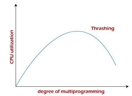
Working Set:

• The working set of a process is the subset of its pages that are actively being used during a given time interval.
• If the total working set of all processes exceeds the system’s available memory, thrashing is likely to occur.

Causes of Thrashing

1. Insufficient Physical Memory:
   • When the total memory demand of all running processes exceeds the available physical memory, pages must be constantly swapped between RAM and disk.
2. High Multiprogramming Level:
   • Increasing the degree of multiprogramming (i.e., the number of concurrent processes) without adequate physical memory can lead to thrashing. Each process competes for memory, and the system cannot maintain the working set for each process in RAM.
3. Poorly Designed Page Replacement Algorithms:
   • Inefficient page replacement algorithms can exacerbate thrashing by frequently removing pages that will soon be needed again.
4. Large Processes or Data Sets:
   • Processes that require large amounts of memory can induce thrashing if the memory demand is not met.
5. System Load Changes:
   • Sudden changes in the workload, such as starting several large processes at once, can lead to thrashing if the system cannot accommodate the increased memory demand.

Effects of Thrashing

1. Decreased System Performance:
   • The CPU is heavily utilized for handling page faults and performing disk I/O operations, leaving little time for actual computation.
2. Increased Latency:
   • The response time for applications becomes significantly longer as the system struggles to load required pages into memory.
3. Higher Disk Activity:
   • Excessive paging leads to increased disk access, which can wear out disk drives over time and further slow down the system.
4. Lower Throughput:
   • The overall throughput of the system decreases as fewer processes can be effectively executed within a given time frame.
5. Unresponsive Applications:
   • Applications may become unresponsive or exhibit erratic behavior as they continually wait for pages to be loaded from disk

Example of Thrashing

Scenario:

Consider a system with 4 GB of RAM running multiple applications simultaneously, each with significant memory requirements.

• Applications:
  • App A: Requires 1 GB of RAM
  • App B: Requires 1.5 GB of RAM
  • App C: Requires 1.2 GB of RAM
  • App D: Requires 1.5 GB of RAM

Total Memory Demand: 1 GB + 1.5 GB + 1.2 GB + 1.5 GB = 5.2 GB

Since the total memory demand (5.2 GB) exceeds the available RAM (4 GB), the system must constantly swap pages to keep the applications running.

Impact:

• The CPU spends more time handling page faults than executing application code.
• Disk I/O operations increase as pages are frequently swapped between RAM and disk.
• Applications become unresponsive or slow, and overall system performance degrades.

Mitigation:

• Increase RAM: Adding more RAM to the system can accommodate the memory demand of all applications.
• Limit Applications: Reducing the number of running applications can ensure that the working set fits within available memory.
• Optimize Applications: Optimizing memory usage in applications can reduce their memory footprint.

Conclusion

Thrashing is a critical performance issue that can severely degrade system performance and user experience. By understanding its causes and implementing strategies to mitigate its effects, systems can achieve better performance and stability. Proper memory management and optimization play a key role in preventing thrashing and maintaining efficient operation in computing environments.

Cause of Thrashing

Thrashing in an operating system is a performance issue that occurs when the system spends a significant amount of time swapping pages between the main memory and disk, rather than executing the actual processes. This leads to high disk I/O activity and reduced overall performance. Let’s delve into the main causes of thrashing:

Causes of Thrashing

1. Insufficient Physical Memory

• Description:
  • When the total memory demand of running processes exceeds the available physical memory (RAM), the system must frequently swap pages in and out to keep processes running.
  • As more processes are loaded into memory than it can handle, this leads to continuous page replacement and swapping.
• Example:
  • Consider a system with 4 GB of RAM running several applications simultaneously, each requiring a substantial amount of memory. If the combined memory requirement of these applications exceeds 4 GB, the system will be forced to swap pages frequently, leading to thrashing.

2. High Degree of Multiprogramming

• Description:
  • Increasing the degree of multiprogramming (i.e., the number of processes in memory at the same time) without sufficient memory can cause thrashing.
  • Each process needs a certain number of pages to execute efficiently (its working set). If too many processes are loaded, there might not be enough memory to hold each process’s working set.
• Example:
  • If a system is configured to handle 10 concurrent processes efficiently, but 20 processes are loaded, the memory demand can overwhelm the available RAM, leading to excessive paging.

3. Poorly Designed Page Replacement Algorithms

• Description:
  • Inefficient page replacement algorithms can exacerbate thrashing by frequently removing pages that are still in use or will soon be used again.
  • Algorithms that do not consider the frequency and recency of page usage might swap out critical pages, causing more page faults.
• Example:
  • Using a simple page replacement algorithm like FIFO (First-In, First-Out) without considering page access patterns can lead to high page fault rates, as frequently used pages might be swapped out prematurely.

4. Large Processes or Working Sets

• Description:
  • Large processes with significant memory requirements can lead to thrashing if the system cannot allocate sufficient memory to hold the entire working set of each process.
  • Applications that use large data sets or have complex operations can quickly exceed available memory resources.
• Example:
  • A large database application that requires a significant portion of memory for its operations can cause thrashing if the system does not have enough RAM to accommodate its entire working set.

5. Frequent Context Switching

• Description:
  • Rapid switching between processes (context switching) can increase the frequency of page faults, especially if the working sets of the processes are not fully resident in memory.
  • Each switch may require loading pages from disk if the new process’s pages have been swapped out.
• Example:
  • In a multi-tasking environment, frequent switching between several memory-intensive applications can lead to thrashing if the system cannot keep all necessary pages in RAM.

6. Dynamic Changes in Process Behavior

• Description:
  • Processes that dynamically change their memory usage patterns can cause sudden spikes in memory demand, leading to thrashing.
  • Unexpected workload increases or changes in application behavior can disrupt memory allocation.
• Example:
  • A process that suddenly loads a large dataset or spawns additional threads may require more memory than initially allocated, causing thrashing as the system struggles to keep up with the demand.

7. Lack of Adequate Swap Space

• Description:
  • Insufficient swap space on the disk can exacerbate thrashing, as the system has limited space to store swapped-out pages.
  • A lack of swap space can lead to situations where the system cannot accommodate all necessary page swaps, leading to even more frequent page faults.
• Example:
  • A system with limited disk space for swapping might experience thrashing when running multiple large applications, as there is no room to store all the swapped-out pages.