
Introduction
Data structures are essential concepts in computer science and programming, providing ways to store, organize, and manage data efficiently. When implemented using the C programming language, data structures enable the development of efficient algorithms and systems.
Data structures in C are fundamental to organizing and managing data efficiently. By selecting the appropriate data structure, you can solve complex problems in programming and design efficient algorithms. Understanding these structures and their real-life applications can significantly enhance your ability to design and implement software systems.
Data Structure:
A data structure is a storage that is used to store and organize data. It is a way of arranging data on a computer so that it can be accessed and updated efficiently.
Data structures are an integral part of computers used for the arrangement of data in memory. They are essential and responsible for organizing, processing, accessing, and storing data efficiently.
Need Of Data structure :
The structure of the data and the synthesis of the algorithm are relative to each other. Data presentation must be easy to understand so the developer, as well as the user, can make an efficient implementation of the operation.
Data structures provide an easy way of organizing, retrieving, managing, and storing data.
Here is a list of the needs for data.
- Data structure modification is easy.
- It requires less time.
- Save storage memory space.
- Data representation is easy.
- Easy access to the large database.
Types of Data Structures in C
1. Linear Data Structures
Linear data structures arrange data in a sequential manner, where each element is connected to its previous and next element. They are simple and easy to implement, making them suitable for straightforward data storage and retrieval operations.
Example: Linked list, Stack, Oueue, and Array
2. Non-Linear Data Structures
Non-linear data structures arrange data hierarchically, allowing for more complex relationships between elements. These structures are suitable for representing complex relationships and solving advanced problems.
Example: Trees and Graphs
Classification of Data Structure:
Data structures can be classified into several categories based on how they organize and manage data. Understanding these classifications helps in selecting the appropriate data structure for a given problem.
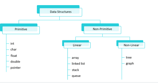
1. Primitive Data Structures
Primitive data structures are the basic building blocks provided by a programming language. They are simple and directly supported by the language.
- Examples:
- Integer: Used for numerical data.
- Float: Used for decimal numbers.
- Character: Used for single characters.
- Boolean: Used for true/false values.
2. Non-Primitive Data Structures
Non-primitive data structures are more complex and can be built using primitive data types. They are used to store and manage large amounts of data efficiently.
Linear Data Structures
Linear data structures organize data in a sequential manner. Each element is connected to the next, allowing for straightforward traversal and management.
- Arrays: A collection of elements of the same type, stored in contiguous memory locations. They allow fast access using indices.
- Linked Lists: A series of nodes, where each node contains data and a pointer to the next node. They allow dynamic memory allocation.
- Doubly Linked List: Each node points to both the previous and next nodes.
- Circular Linked List: The last node points back to the first node, forming a loop.
- Stacks: A stack is a linear data structure that follows the Last In, First Out (LIFO) principle. It allows operations at one end only, called the top.
- Queues: A queue is a linear data structure that follows the First In, First Out (FIFO) principle. It allows operations at both ends: enqueue (insertion) at the rear and dequeue (removal) from the front.
Non-Linear Data Structures
Non-linear data structures organize data hierarchically or graphically, allowing for more complex relationships between elements. These structures are suitable for representing complex data and solving advanced problems.
- Trees: A tree is a hierarchical data structure consisting of nodes connected by edges. It starts with a root node and has zero or more child nodes.
- Graphs: A graph is a collection of nodes (vertices) and edges connecting pairs of nodes. It can be directed or undirected.
data types and abstract data types
Data Types
A data type is a classification that specifies which type of value a variable can hold in programming. Each data type has a predefined set of operations that can be performed on it. Data types are generally divided into two categories:
1. Primitive Data Types
These are the basic building blocks for data manipulation and are usually built into the language. Common primitive data types include:
- Integer: Represents whole numbers (e.g., -3, 0, 42).
- Float/Double: Represents real numbers or numbers with decimal points (e.g., 3.14, -0.001).
- Character: Represents single characters (e.g., ‘a’, ‘B’, ‘@’).
- Boolean: Represents true or false values.
Abstract Data Types (ADTs)
An abstract data type (ADT) is a theoretical concept used to define data types by their behavior from the point of view of a user, specifically in terms of possible values and operations on that data type, without specifying implementation details. ADTs are about the what and how of data interaction, not the how it is implemented.
Common Abstract Data Types
- List:
- Description: An ordered collection of elements.
- Operations: Add, remove, get, set, search, etc.
- Examples: ArrayList in Java, List in Python.
- Stack:
- Description: A collection of elements that follows the Last-In-First-Out (LIFO) principle.
- Operations: Push (add), pop (remove), peek (view top element), isEmpty.
- Examples: Call stack, undo mechanisms in applications.
- Queue:
- Description: A collection of elements that follows the First-In-First-Out (FIFO) principle.
- Operations: Enqueue (add), dequeue (remove), front (view first element), isEmpty.
- Examples: Print queue, task scheduling.
- Tree:
- Description: A hierarchical structure with a root element and sub-elements, represented as nodes.
- Operations: Insert, delete, traverse (preorder, inorder, postorder), search.
- Examples: File system hierarchy, DOM in HTML.
- Graph:
- Description: A set of nodes connected by edges.
- Operations: Add/remove nodes/edges, traverse (BFS, DFS), find path/cycle.
- Examples: Social network connections, route maps.
- Hash Table:
- Description: A collection that maps keys to values using a hash function.
- Operations: Insert, delete, search by key.
- Examples: Dictionary in Python, HashMap in Java.
Why Use Abstract Data Types?
- Abstraction: ADTs allow you to focus on the logic of your application without worrying about the underlying implementation.
- Modularity: ADTs enable modular code, which is easier to maintain and understand.
- Reusability: Once implemented, an ADT can be reused across different programs.
- Flexibility: You can change the underlying implementation without affecting code that uses the ADT, as long as the interface remains the same.
Summary
- Data Types are fundamental to understanding what kind of data you can work with in a programming language.
- Abstract Data Types (ADTs) allow you to abstract the complexity of data structures and focus on their behavior rather than their implementation.
Space and Time Comlexities
Time Complexity
Time complexity refers to the amount of time an algorithm takes to complete as a function of the length of the input. It gives an upper bound on the running time of an algorithm, and is usually expressed using Big O notation.
Space Complexity
Space complexity refers to the amount of memory an algorithm requires as a function of the length of the input. It includes both the space needed for the input data and the additional space required by the algorithm itself.
Components of Space Complexity
- Fixed Part:
- Memory space required by variables, constants, and program code, which doesn’t change with input size.
- Variable Part:
- Memory space required dynamically based on input size, such as:
- Auxiliary Space: Extra space or temporary space used by an algorithm.
- Input Space: Space required to store the input data.
- Memory space required dynamically based on input size, such as:
Searching and Sorting
Sorting is a fundamental operation in computer science and data structures. It involves arranging the elements of a list or array in a specific order, typically in ascending or descending order. Sorting is essential for optimizing the performance of other algorithms, such as searching and data retrieval, and it has numerous practical applications in real-world problems.
Why Sorting is Important
- Search Optimization: Sorted data allows for faster searching techniques like binary search, which significantly reduces the search time.
- Data Processing: Sorted data can make it easier to detect duplicates, find extremes (minimum or maximum values), and analyze data patterns.
- Efficiency in Algorithms: Many algorithms, such as merge sort and quicksort, rely on sorting as a foundational step.
- Data Presentation: Sorting helps in presenting data in a more readable and organized manner.
Sorting Algorithms:
1.Bubble sort
2.Selection sort
3.Insertion sort
4.Quick sort
5.Merge sort
1.Bubble Sort
Bubble Sort is the simplest sorting that works by repeatedly swapping the adjacent elements if they are in the wrong order. This algorithm is not suitable for large data sets as its average and worst-case time complexity is quite high.
In Bubble Sort algorithm,
This process is then continued to find the second largest and place it and so on until the data is sorted.
traverse from left and compare adjacent elements and the higher one is placed at right side.
In this way, the largest element is moved to the rightmost end at first.
Working of Bubble Sort
Suppose we are trying to sort the elements in ascending order.
1. First Iteration (Compare and Swap)
- Starting from the first index, compare the first and the second elements.
- If the first element is greater than the second element, they are swapped.
- Now, compare the second and the third elements. Swap them if they are not in order.
- The above process goes on until the last element.

2. Remaining Iteration
The same process goes on for the remaining iterations.
After each iteration, the largest element among the unsorted elements is placed at the end.

The array is sorted when all the unsorted elements are placed at their correct positions.
The array is sorted if all elements are kept in the right order

Bubble sort program in c
#include <stdio.h>
// Function to perform Bubble Sort
void bubble_sort(int arr[], int n) {
    int i, j, temp;
    int swapped;

    // Loop through each pass
    for (i = 0; i < n - 1; i++) {
        swapped = 0;  // Initialize the swapped flag

        // Traverse the array from 0 to n-i-1
        for (j = 0; j < n - i - 1; j++) {
            // Compare adjacent elements
            if (arr[j] > arr[j + 1]) {
                // Swap if the current element is greater than the next element
                temp = arr[j];
                arr[j] = arr[j + 1];
                arr[j + 1] = temp;
                swapped = 1;  // Set the swapped flag to true
            }
        }

        // If no elements were swapped, the array is sorted
        if (swapped == 0) {
            break;
        }
    }
}

// Function to print the array
void print_array(int arr[], int size) {
    int i;
    for (i = 0; i < size; i++) {
        printf("%d ", arr[i]);
    }
    printf("\n");
}

// Main function to test Bubble Sort
int main() {
    int arr[] = {64, 34, 25, 12, 22, 11, 90};
    int n = sizeof(arr) / sizeof(arr[0]);

    printf("Unsorted array: ");
    print_array(arr, n);

    bubble_sort(arr, n);

    printf("Sorted array: ");
    print_array(arr, n);

    return 0;
}
–>Click here for detailed explanation of Bubble sort program
1. Include Header File
#include <stdio.h>#include <stdio.h>: This header file is included to allow the use of input and output functions likeprintf().
2. Bubble Sort Function
void bubble_sort(int arr[], int n) {
    int i, j, temp;
    int swapped;
- Function Signature:
void bubble_sort(int arr[], int n)– This function sorts an arrayarrof sizenusing the Bubble Sort algorithm. - Local Variables:
int i, j, temp;: Loop indices and a temporary variable for swapping.int swapped;: A flag to track if any elements were swapped during the pass.
 for (i = 0; i < n - 1; i++) {
        swapped = 0;  // Initialize the swapped flag

        for (j = 0; j < n - i - 1; j++) {
            if (arr[j] > arr[j + 1]) {
                temp = arr[j];
                arr[j] = arr[j + 1];
                arr[j + 1] = temp;
                swapped = 1;  // Set the swapped flag to true
            }
        }

        if (swapped == 0) {
            break;
        }
    }
}
- Outer Loop (
for (i = 0; i < n - 1; i++)):- Runs
n - 1times, wherenis the number of elements in the array. - Each pass ensures that the largest unsorted element is moved to its correct position.
- Runs
- Inner Loop (
for (j = 0; j < n - i - 1; j++)):- Compares each pair of adjacent elements.
n - i - 1is used because afteripasses, the lastielements are sorted and in their correct positions.
- Swapping Elements:
- If
arr[j] > arr[j + 1], swap them using the temporary variabletemp. - Set
swapped = 1to indicate that a swap has occurred.
- If
- Early Termination:
- If no elements were swapped during the pass (
swapped == 0), break out of the loop early as the array is already sorted.
- If no elements were swapped during the pass (
3. Print Array Function
void print_array(int arr[], int size) {
    int i;
    for (i = 0; i < size; i++) {
        printf("%d ", arr[i]);
    }
    printf("\n");
}
- Function Signature:
void print_array(int arr[], int size)– This function prints the elements of an arrayarrof sizesize. - Loop (
for (i = 0; i < size; i++)):- Iterates through the array and prints each element.
printf("\n");: Prints a newline character after the array elements.
4. Main Function
int main() {
    int arr[] = {64, 34, 25, 12, 22, 11, 90};
    int n = sizeof(arr) / sizeof(arr[0]);

    printf("Unsorted array: ");
    print_array(arr, n);

    bubble_sort(arr, n);

    printf("Sorted array: ");
    print_array(arr, n);

    return 0;
}
- Array Initialization:
int arr[] = {64, 34, 25, 12, 22, 11, 90};– Initializes an array with unsorted integers. - Size Calculation:
int n = sizeof(arr) / sizeof(arr[0]);– Calculates the number of elements in the array. - Print Unsorted Array:
print_array(arr, n);– Prints the array before sorting. - Sort Array:
bubble_sort(arr, n);– Calls the Bubble Sort function to sort the array. - Print Sorted Array:
print_array(arr, n);– Prints the array after sorting.
Summary
- Bubble Sort is a simple sorting algorithm that repeatedly compares and swaps adjacent elements to sort the array.
- Time Complexity: O(n²) in the average and worst cases, making it inefficient for large datasets.
- Space Complexity: O(1) – Bubble Sort is an in-place sorting algorithm.
- Optimization: The algorithm can terminate early if no swaps are made in a pass.
This program provides a clear and practical example of how Bubble Sort works, demonstrating its basic functionality and the steps involved in sorting an array.
Selection Sort
The algorithm repeatedly selects the smallest (or largest) element from the unsorted portion of the list and swaps it with the first element of the unsorted part. This process is repeated for the remaining unsorted portion until the entire list is sorted.
Working of Selection Sort
- Set the first element as
minimum.

2.Compare minimum with the second element. If the second element is smaller than minimum, assign the second element as minimum.
Compare minimum with the third element. Again, if the third element is smaller, then assign minimum to the third element otherwise do nothing. The process goes on until the last element.

3.After each iteration, minimum is placed in the front of the unsorted list.

4.For each iteration, indexing starts from the first unsorted element. Step 1 to 3 are repeated until all the elements are placed at their correct positions.


Selection Sort program in C
#include <stdio.h>
void selectionSort(int arr[], int n) {
    int i, j, min_idx, temp;
    for (i = 0; i < n - 1; i++) {
        min_idx = i;
        for (j = i + 1; j < n; j++) {
            if (arr[j] < arr[min_idx]) {
                min_idx = j;
            }
        }
        if (min_idx != i) {
            temp = arr[i];
            arr[i] = arr[min_idx];
            arr[min_idx] = temp;
        }
    }
}

void printArray(int arr[], int size) {
    int i;
    for (i = 0; i < size; i++) {
        printf("%d ", arr[i]);
    }
    printf("\n");
}

int main() {
    int arr[] = {64, 25, 12, 22, 11};
    int n = sizeof(arr) / sizeof(arr[0]);

    printf("Original array: \n");
    printArray(arr, n);

    selectionSort(arr, n);

    printf("Sorted array: \n");
    printArray(arr, n);

    return 0;
}
–>Click here for detailed explanation of Selection sort program
1. Function to Perform Selection Sort
void selectionSort(int arr[], int n) {
    int i, j, min_idx, temp;

    // Traverse through all array elements
    for (i = 0; i < n - 1; i++) {
        // Find the minimum element in the remaining unsorted array
        min_idx = i;
        for (j = i + 1; j < n; j++) {
            if (arr[j] < arr[min_idx]) {
                min_idx = j;
            }
        }

        // Swap the found minimum element with the first element
        if (min_idx != i) {
            temp = arr[i];
            arr[i] = arr[min_idx];
            arr[min_idx] = temp;
        }
    }
}
Explanation:
- Initialization:
iandjare loop variables.min_idxholds the index of the minimum element found in the unsorted part.tempis used for swapping elements.
- Outer Loop (
for (i = 0; i < n - 1; i++)):- Iterates through each element from the start up to the second-to-last element (since the last element will be sorted by the time the loop finishes).
- Inner Loop (
for (j = i + 1; j < n; j++)):- Finds the minimum element from the sub-array starting at
i + 1ton.
- Finds the minimum element from the sub-array starting at
- Finding Minimum:
- If
arr[j] < arr[min_idx], updatemin_idxtoj.
- If
- Swapping:
- After finding the minimum element in the unsorted part, swap it with the element at index
i.
- After finding the minimum element in the unsorted part, swap it with the element at index
2. Function to Print the Array
void printArray(int arr[], int size) {
    int i;
    for (i = 0; i < size; i++) {
        printf("%d ", arr[i]);
    }
    printf("\n");
}
Explanation:
- Iterates over the array and prints each element followed by a space.
printf("\n");adds a newline at the end of the array printout.
3. Main Function
int main() {
    int arr[] = {64, 25, 12, 22, 11};
    int n = sizeof(arr) / sizeof(arr[0]);

    printf("Original array: \n");
    printArray(arr, n);

    selectionSort(arr, n);

    printf("Sorted array: \n");
    printArray(arr, n);

    return 0;
}
Explanation:
Calls printArray to display the sorted array.
Array Initialization:
An array arr is initialized with some values.
Calculate Array Size:
n is computed as the total number of elements in the array using sizeof(arr) / sizeof(arr[0]).
Print Original Array:
Calls printArray to display the unsorted array.
Sort Array:
Calls selectionSort to sort the array.
Print Sorted Array:
Insertion Sort Algorithm:
Insertion sort is a simple sorting algorithm that works by building a sorted array one element at a time. It is considered an ” in-place ” sorting algorithm, meaning it doesn’t require any additional memory space beyond the original array.Insertion sort is a simple sorting algorithm that works by iteratively inserting each element of an unsorted list into its correct position in a sorted portion of the list. It is a stable sorting algorithm, meaning that elements with equal values maintain their relative order in the sorted output.
Working of Insertion Sort
Suppose we need to sort the following array.

1.The first element in the array is assumed to be sorted. Take the second element and store it separately in key.
Compare key with the first element. If the first element is greater than key, then key is placed in front of the first element.

2.Now, the first two elements are sorted.
Take the third element and compare it with the elements on the left of it. Placed it just behind the element smaller than it. If there is no element smaller than it, then place it at the beginning of the array.

3.Similarly, place every unsorted element at its correct position.


Insertion Sort program in C
#include <stdio.h>
void insertionSort(int arr[], int n) {
    int i, key, j;
    for (i = 1; i < n; i++) {
        key = arr[i]; // The element to be inserted
        j = i - 1;

        while (j >= 0 && arr[j] > key) {
            arr[j + 1] = arr[j];
            j = j - 1;
        }

        arr[j + 1] = key;
    }
}

void printArray(int arr[], int size) {
    int i;
    for (i = 0; i < size; i++) {
        printf("%d ", arr[i]);
    }
    printf("\n");
}

int main() {
    int arr[] = {64, 25, 12, 22, 11};
    int n = sizeof(arr) / sizeof(arr[0]);

    printf("Original array: \n");
    printArray(arr, n);

    insertionSort(arr, n);

    printf("Sorted array: \n");
    printArray(arr, n);

    return 0;
}
–>Click here for detailed explanation of insertion sort program
Function insertionSort:
cCopy codevoid insertionSort(int arr[], int n) {
    int i, key, j;

    // Traverse through 1 to n-1
    for (i = 1; i < n; i++) {
        key = arr[i]; // The element to be inserted
        j = i - 1;

        // Move elements that are greater than key to one position ahead
        while (j >= 0 && arr[j] > key) {
            arr[j + 1] = arr[j];
            j = j - 1;
        }

        // Place the key at after the last shifted element
        arr[j + 1] = key;
    }
}
Explanation:
- Initialization:
iis the index for the current element being inserted.keyis the element to be inserted into the sorted portion of the array.jis used to find the correct position forkeyin the sorted portion.
- Outer Loop (
for (i = 1; i < n; i++)):- Iterates from the second element to the last element.
keyis set to the current elementarr[i].
- Inner Loop (
while (j >= 0 && arr[j] > key)):- Compares
keywith elements in the sorted portion (i.e., elements before indexi). - Shifts elements greater than
keyone position to the right.
- Compares
- Insertion:
- Once the correct position is found,
keyis placed in its correct position (arr[j + 1]).
- Once the correct position is found,
Function printArray:
cCopy codevoid printArray(int arr[], int size) {
    int i;
    for (i = 0; i < size; i++) {
        printf("%d ", arr[i]);
    }
    printf("\n");
}
Explanation:
- Iterates over the array and prints each element followed by a space.
Main Function:
cCopy codeint main() {
    int arr[] = {64, 25, 12, 22, 11};
    int n = sizeof(arr) / sizeof(arr[0]);

    printf("Original array: \n");
    printArray(arr, n);

    insertionSort(arr, n);

    printf("Sorted array: \n");
    printArray(arr, n);

    return 0;
}
Explanation:
Prints the sorted array.
Initializes an array and computes its size.
Prints the original unsorted array.
Calls insertionSort to sort the array.
Quick Sort:
Quick Sort is a sorting algorithm based on the Divide and conquer that picks an element as a pivot and partitions the given array around the picked pivot by placing the pivot in its correct position in the sorted array.
Steps of Quick Sort
- Choose a Pivot: Select an element from the array to act as the pivot. The choice of the pivot can be based on different strategies, such as picking the first element, the last element, a random element, or the median.
- Partition the Array:
- Rearrange the array so that all elements less than the pivot come before it and all elements greater than the pivot come after it.
- After partitioning, the pivot is in its correct position in the sorted array.
- Recursively Apply:
- Apply the same process to the sub-arrays formed by dividing the array at the pivot.
- Base Case:
- The recursion stops when the sub-array has fewer than two elements, as a single element or an empty array is already sorted.
Working of Quicksort Algorithm
1. Select the Pivot Element
There are different variations of quicksort where the pivot element is selected from different positions. Here, we will be selecting the rightmost element of the array as the pivot element.

2. Rearrange the Array
Now the elements of the array are rearranged so that elements that are smaller than the pivot are put on the left and the elements greater than the pivot are put on the right.

Here’s how we rearrange the array:
- A pointer is fixed at the pivot element. The pivot element is compared with the elements beginning from the first index.

If the element is greater than the pivot element, a second pointer is set for that element.

Now, pivot is compared with other elements. If an element smaller than the pivot element is reached, the smaller element is swapped with the greater element found earlier.

Again, the process is repeated to set the next greater element as the second pointer. And, swap it with another smaller element.

The process goes on until the second last element is reached

Finally, the pivot element is swapped with the second pointer

Divide Subarrays
Pivot elements are again chosen for the left and the right sub-parts separately. And, step 2 is repeated.

Quick Sort Program in C
#include <stdio.h>
void swap(int *a, int *b) {
    int temp = *a;
    *a = *b;
    *b = temp;
}

int partition(int arr[], int low, int high) {
    int pivot = arr[high]; // Choosing the last element as pivot
    int i = (low - 1); // Index of the smaller element

    for (int j = low; j < high; j++) {

        if (arr[j] < pivot) {
            i++; // Increment index of the smaller element
            swap(&arr[i], &arr[j]);
        }
    }

    swap(&arr[i + 1], &arr[high]);
    return (i + 1);
}


void quickSort(int arr[], int low, int high) {
    if (low < high) {

        int pi = partition(arr, low, high);
        quickSort(arr, low, pi - 1);
        quickSort(arr, pi + 1, high);
    }
}


void printArray(int arr[], int size) {
    for (int i = 0; i < size; i++) {
        printf("%d ", arr[i]);
    }
    printf("\n");
}


int main() {
    int arr[] = {10, 7, 8, 9, 1, 5};
    int n = sizeof(arr) / sizeof(arr[0]);

    printf("Original array: \n");
    printArray(arr, n);

    quickSort(arr, 0, n - 1);

    printf("Sorted array: \n");
    printArray(arr, n);

    return 0;
}
–>Click here for detailed explanation of Quick sort program
Function to Swap Elements
void swap(int *a, int *b) {
    int temp = *a;
    *a = *b;
    *b = temp;
}
- Purpose: This function swaps two elements in the array.
- How it Works: It uses a temporary variable
tempto hold one value while swapping the values of the two elements.
2. Partition Function
int partition(int arr[], int low, int high) {
    int pivot = arr[high]; // Choosing the last element as pivot
    int i = (low - 1); // Index of the smaller element

    for (int j = low; j < high; j++) {
        // If current element is smaller than the pivot
        if (arr[j] < pivot) {
            i++; // Increment index of the smaller element
            swap(&arr[i], &arr[j]);
        }
    }
    // Swap the pivot element with the element at index i+1
    swap(&arr[i + 1], &arr[high]);
    return (i + 1);
}
- Purpose: The partition function arranges the elements in such a way that elements less than the pivot are on its left, and elements greater are on its right.
- How it Works:
- Pivot Selection: Here, the pivot is chosen as the last element of the array.
- Partitioning:
- Traverse through the array from
lowtohigh - 1. - If an element is smaller than the pivot, it is swapped with an element on the left of the pivot’s current position.
- Finally, swap the pivot with the element at index
i + 1so that the pivot is in its correct position.
- Traverse through the array from
3. Quick Sort Function
void quickSort(int arr[], int low, int high) {
    if (low < high) {
        // Partitioning index
        int pi = partition(arr, low, high);

        // Recursively sort elements before and after partition
        quickSort(arr, low, pi - 1);
        quickSort(arr, pi + 1, high);
    }
}
- Purpose: This function recursively sorts the array.
- How it Works:
- Base Case: The recursion stops when
lowis not less thanhigh, which means the sub-array has one or zero elements and is already sorted. - Recursion:
- Call
partitionto get the pivot indexpi. - Recursively sort the sub-arrays on the left and right of the pivot.
- Call
- Base Case: The recursion stops when
4. Function to Print the Array
void printArray(int arr[], int size) {
    for (int i = 0; i < size; i++) {
        printf("%d ", arr[i]);
    }
    printf("\n");
}
- Purpose: This function prints the elements of the array.
- How it Works: It iterates through the array and prints each element followed by a space.
5. Main Function
int main() {
    int arr[] = {10, 7, 8, 9, 1, 5}; // Array to be sorted
    int n = sizeof(arr) / sizeof(arr[0]); // Number of elements in the array

    printf("Original array: \n");
    printArray(arr, n);

    quickSort(arr, 0, n - 1); // Sort the array using quick sort

    printf("Sorted array: \n");
    printArray(arr, n); // Print the sorted array

    return 0;
}
Prints the sorted array.
Purpose: This function tests the quick sort implementation.
How it Works:
Initializes an array with values.
Prints the original array.
Calls quickSort to sort the array.
Merge Sort:
Merge sort is a sorting algorithm that follows the divide-and-conquer approach. It works by recursively dividing the input array into smaller subarrays and sorting those subarrays then merging them back together to obtain the sorted array.
In simple terms, we can say that the process of merge sort is to divide the array into two halves, sort each half, and then merge the sorted halves back together. This process is repeated until the entire array is sorted.
Here is the Example:

Divide and Conquer Strategy
Using the Divide and Conquer technique, we divide a problem into subproblems. When the solution to each subproblem is ready, we ‘combine’ the results from the subproblems to solve the main problem.
Suppose we had to sort an array A. A subproblem would be to sort a sub-section of this array starting at index p and ending at index r, denoted as A[p..r].
Divide
If q is the half-way point between p and r, then we can split the subarray A[p..r] into two arrays A[p..q] and A[q+1, r].
Conquer
In the conquer step, we try to sort both the subarrays A[p..q] and A[q+1, r]. If we haven’t yet reached the base case, we again divide both these subarrays and try to sort them.
Combine
When the conquer step reaches the base step and we get two sorted subarrays A[p..q] and A[q+1, r] for array A[p..r], we combine the results by creating a sorted array A[p..r] from two sorted subarrays A[p..q] and A[q+1, r].
Merge Sort program in C
#include <stdio.h>
#include <stdlib.h>

void merge(int arr[], int l, int m, int r) {
    int n1 = m - l + 1;
    int n2 = r - m;

    int *L = (int *)malloc(n1 * sizeof(int));
    int *R = (int *)malloc(n2 * sizeof(int));

    for (int i = 0; i < n1; i++)
        L[i] = arr[l + i];
    for (int j = 0; j < n2; j++)
        R[j] = arr[m + 1 + j];

    int i = 0;
    int j = 0;
    int k = l;
    while (i < n1 && j < n2) {
        if (L[i] <= R[j]) {
            arr[k++] = L[i++];
        } else {
            arr[k++] = R[j++];
        }
    }

    while (i < n1) {
        arr[k++] = L[i++];
    }

    while (j < n2) {
        arr[k++] = R[j++];
    }

    free(L);
    free(R);
}

void mergeSort(int arr[], int l, int r) {
    if (l < r) {
        int m = l + (r - l) / 2;

        mergeSort(arr, l, m);
        mergeSort(arr, m + 1, r);

        merge(arr, l, m, r);
    }
}

void printArray(int arr[], int size) {
    for (int i = 0; i < size; i++) {
        printf("%d ", arr[i]);
    }
    printf("\n");
}

int main() {
    int arr[] = {12, 11, 13, 5, 6, 7};
    int n = sizeof(arr) / sizeof(arr[0]);

    printf("Original array: \n");
    printArray(arr, n);

    mergeSort(arr, 0, n - 1);

    printf("Sorted array: \n");
    printArray(arr, n);

    return 0;
}
–>Click here for detailed explanation of Merge sort program
Merge Function
void merge(int arr[], int l, int m, int r) {
    int n1 = m - l + 1;
    int n2 = r - m;

    int *L = (int *)malloc(n1 * sizeof(int));
    int *R = (int *)malloc(n2 * sizeof(int));

    for (int i = 0; i < n1; i++)
        L[i] = arr[l + i];
    for (int j = 0; j < n2; j++)
        R[j] = arr[m + 1 + j];

    int i = 0;
    int j = 0;
    int k = l;
    while (i < n1 && j < n2) {
        if (L[i] <= R[j]) {
            arr[k++] = L[i++];
        } else {
            arr[k++] = R[j++];
        }
    }

    while (i < n1) {
        arr[k++] = L[i++];
    }

    while (j < n2) {
        arr[k++] = R[j++];
    }

    free(L);
    free(R);
}
- Purpose: Merges two sorted sub-arrays into a single sorted array.
- How it Works:
- Temporary Arrays: Create temporary arrays
LandRto hold the elements of the left and right sub-arrays. - Copy Elements: Copy the elements of the sub-arrays into
LandR. - Merge: Merge the elements back into the original array by comparing elements of
LandR. - Copy Remaining Elements: Copy any remaining elements from
LorR(if any).
- Temporary Arrays: Create temporary arrays
2. Merge Sort Function
void mergeSort(int arr[], int l, int r) {
    if (l < r) {
        int m = l + (r - l) / 2;

        mergeSort(arr, l, m);
        mergeSort(arr, m + 1, r);

        merge(arr, l, m, r);
    }
}
- Purpose: Recursively sorts the array using merge sort.
- How it Works:
- Base Case: If
lis not less thanr, the array has one or zero elements and is already sorted. - Divide: Find the middle index
m. - Recursive Sort: Recursively sort the two halves of the array.
- Merge: Merge the sorted halves.
- Base Case: If
3. Function to Print the Array
void printArray(int arr[], int size) {
    for (int i = 0; i < size; i++) {
        printf("%d ", arr[i]);
    }
    printf("\n");
}
- Purpose: Prints the elements of the array.
- How it Works: Iterates through the array and prints each element followed by a space.
4. Main Function
int main() {
    int arr[] = {12, 11, 13, 5, 6, 7};
    int n = sizeof(arr) / sizeof(arr[0]);

    printf("Original array: \n");
    printArray(arr, n);

    mergeSort(arr, 0, n - 1);

    printf("Sorted array: \n");
    printArray(arr, n);

    return 0;
}
Prints the sorted array.
Purpose: Tests the merge sort implementation.
How it Works:
Initializes an array with values.
Prints the original array.
Calls mergeSort to sort the array.
Searching
Searching is the process of locating a specific record or element within a large dataset. This can involve searching through various data structures like arrays, linked lists, trees, heaps, and graphs. As data sizes grow, multiple techniques and algorithms are used to perform efficient searches.
Types of Searching :
1.Binary search
2.linear search
Linear Search:
The linear search algorithm is defined as a sequential search algorithm that starts at one end and goes through each element of a list until the desired element is found; otherwise, the search continues till the end of the dataset. In this article, we will learn about the basics of the linear search algorithm, its applications, advantages, disadvantages, and more to provide a deep understanding of linear search.
Linear Search Algorithm
Start from the first element of the array.
Compare each element with the target value.
If a match is found, return the index of the element.
If no match is found by the end of the list, return a value indicating the element is not present (e.g., -1).
Linear Search program in c
#include <stdio.h>

int linearSearch(int arr[], int size, int target) {
    for (int i = 0; i < size; i++) {
        if (arr[i] == target) {
            return i;
        }
    }
    return -1;
}

void printArray(int arr[], int size) {
    for (int i = 0; i < size; i++) {
        printf("%d ", arr[i]);
    }
    printf("\n");
}

int main() {
    int arr[] = {5, 3, 7, 2, 8, 6};
    int size = sizeof(arr) / sizeof(arr[0]);
    int target = 8;

    printf("Array: ");
    printArray(arr, size);

    int result = linearSearch(arr, size, target);
    if (result != -1) {
        printf("Element %d found at index %d\n", target, result);
    } else {
        printf("Element %d not found\n", target);
    }

    return 0;
}
–>Click here for detailed explanation of Linear search program
Include Header File
#include <stdio.h>
- Includes the standard input/output library, which is necessary for using
printfand other I/O functions.
2. Linear Search Function
int linearSearch(int arr[], int size, int target) {
    for (int i = 0; i < size; i++) {
        if (arr[i] == target) {
            return i;
        }
    }
    return -1;
}
- Purpose: Searches for a specific value (
target) in an array (arr) and returns its index if found. If the value is not present, it returns-1. - Parameters:
arr[]: The array to be searched.size: The number of elements in the array.target: The value to search for.
- Process:
- Loop: Iterates through each element of the array.
- Comparison: Checks if the current element (
arr[i]) matches thetarget. - Return Index: If a match is found, returns the index of that element.
- Return -1: If no match is found after the loop completes, returns
-1.
3. Print Array Function
void printArray(int arr[], int size) {
    for (int i = 0; i < size; i++) {
        printf("%d ", arr[i]);
    }
    printf("\n");
}
- Purpose: Prints the elements of the array in a single line.
- Parameters:
arr[]: The array to be printed.size: The number of elements in the array.
- Process:
- Loop: Iterates through each element of the array.
- Print Elements: Prints each element followed by a space.
- Newline: After printing all elements, outputs a newline for formatting.
4. Main Function
int main() {
    int arr[] = {5, 3, 7, 2, 8, 6};
    int size = sizeof(arr) / sizeof(arr[0]);
    int target = 8;

    printf("Array: ");
    printArray(arr, size);

    int result = linearSearch(arr, size, target);
    if (result != -1) {
        printf("Element %d found at index %d\n", target, result);
    } else {
        printf("Element %d not found\n", target);
    }

    return 0;
}
Purpose: Serves as the entry point of the program where the array is defined, and the linear search function is tested.
Process:
Array Initialization: Defines an array arr with some values and sets the target value to search for.
Calculate Size: Uses sizeof(arr) / sizeof(arr[0]) to determine the number of elements in the array.
Print Array: Calls printArray to display the array.
Call Linear Search: Invokes linearSearch with the array, size, and target value, and stores the result.
Output Result: Prints whether the target value was found and its index, or indicates that the value was not found.
Binary search
Binary search is an efficient algorithm used to find the position of a target value within a sorted array. It works by repeatedly dividing the search interval in half, which makes it much faster than linear search for large datasets.
Binary Search Algorithm
- Start with the Entire Array:
- Initialize two pointers,
lowandhigh, to represent the current search interval.lowstarts at the beginning of the array, andhighstarts at the end.
- Initialize two pointers,
- Find the Middle Element:
- Calculate the middle index using the formula:
mid = low + (high - low) / 2.
- Calculate the middle index using the formula:
- Compare the Middle Element:
- If the middle element is equal to the target value, the search is complete, and the index of the middle element is returned.
- If the target value is less than the middle element, narrow the search interval to the left half of the array by updating
hightomid - 1. - If the target value is greater than the middle element, narrow the search interval to the right half of the array by updating
lowtomid + 1.
- Repeat:
- Continue steps 2 and 3 until the target value is found or the search interval is empty (
lowexceedshigh).
- Continue steps 2 and 3 until the target value is found or the search interval is empty (
- End of Search:
- If the target value is not found by the time the interval is empty, return a value indicating that the target is not present (e.g.,
-1).
- If the target value is not found by the time the interval is empty, return a value indicating that the target is not present (e.g.,
Binary Search program in c
#include <stdio.h>

int binarySearch(int arr[], int size, int target) {
    int low = 0;
    int high = size - 1;

    while (low <= high) {
        int mid = low + (high - low) / 2;

        if (arr[mid] == target) {
            return mid;
        } else if (arr[mid] < target) {
            low = mid + 1;
        } else {
            high = mid - 1;
        }
    }
    return -1;
}

void printArray(int arr[], int size) {
    for (int i = 0; i < size; i++) {
        printf("%d ", arr[i]);
    }
    printf("\n");
}

int main() {
    int arr[] = {2, 4, 6, 8, 10, 12};
    int size = sizeof(arr) / sizeof(arr[0]);
    int target = 8;

    printf("Array: ");
    printArray(arr, size);

    int result = binarySearch(arr, size, target);
    if (result != -1) {
        printf("Element %d found at index %d\n", target, result);
    } else {
        printf("Element %d not found\n", target);
    }

    return 0;
}
–>Click here for detailed explanation of Binary search program
Binary Search Function
int binarySearch(int arr[], int size, int target) {
    int low = 0;
    int high = size - 1;

    while (low <= high) {
        int mid = low + (high - low) / 2;

        if (arr[mid] == target) {
            return mid;
        } else if (arr[mid] < target) {
            low = mid + 1;
        } else {
            high = mid - 1;
        }
    }
    return -1;
}
- Parameters:
arr[]: The sorted array to be searched.size: The number of elements in the array.target: The value to search for.
- Process:
- Initialize Pointers:
lowstarts at the beginning of the array (0).highstarts at the end of the array (size - 1).
- While Loop:
- Continues as long as
lowis less than or equal tohigh.
- Continues as long as
- Calculate Middle Index:
mid = low + (high - low) / 2to avoid potential overflow.
- Comparison:
- If
arr[mid]equalstarget, returnmid(index of the target). - If
arr[mid]is less thantarget, adjustlowtomid + 1to search the right half. - If
arr[mid]is greater thantarget, adjusthightomid - 1to search the left half.
- If
- Return -1:
- If the target is not found by the end of the loop, return
-1.
- If the target is not found by the end of the loop, return
- Initialize Pointers:
2. Print Array Function
void printArray(int arr[], int size) {
    for (int i = 0; i < size; i++) {
        printf("%d ", arr[i]);
    }
    printf("\n");
}
- Purpose: Prints all the elements of the array in a single line.
- Process:
- Iterates through each element of the array and prints it followed by a space.
- After printing all elements, outputs a newline character.
3. Main Function
int main() {
    int arr[] = {2, 4, 6, 8, 10, 12}; // Sorted array
    int size = sizeof(arr) / sizeof(arr[0]);
    int target = 8;

    printf("Array: ");
    printArray(arr, size);

    int result = binarySearch(arr, size, target);
    if (result != -1) {
        printf("Element %d found at index %d\n", target, result);
    } else {
        printf("Element %d not found\n", target);
    }

    return 0;
}
Array Initialization: Defines a sorted array arr and sets a target value to search for.
Calculate Size: Computes the number of elements in the array using sizeof(arr) / sizeof(arr[0]).
Print Array: Displays the contents of the array using printArray.
Call Binary Search: Searches for the target value in the array and stores the result.
Output Result: Prints whether the target was found and its index, or indicates that the target was not found.
Difference between Binary search and Linear search
| Aspect | Binary Search | Linear Search |
|---|---|---|
| Definition | An efficient algorithm for finding a target in a sorted array by repeatedly dividing the search interval in half. | A simple algorithm for finding a target by sequentially checking each element in the array. |
| Array Requirement | Requires the array to be sorted. | Does not require the array to be sorted. |
| Time Complexity | O(logn)O(\log n)O(logn), where nnn is the number of elements. | O(n)O(n)O(n), where nnn is the number of elements. |
| Space Complexity | O(1)O(1)O(1) for iterative, O(logn)O(\log n)O(logn) for recursive (due to function call stack). | O(1)O(1)O(1). |
| Search Method | Divides the search interval in half repeatedly. | Checks each element one by one. |
| Efficiency | Much more efficient for large datasets due to logarithmic time complexity. | Less efficient for large datasets due to linear time complexity. |
| Implementation | Requires calculating the middle index and adjusting search boundaries. | Simple iteration through the array. |
| Best Case Time Complexity | O(1)O(1)O(1) (if the target is at the middle index). | O(1)O(1)O(1) (if the target is at the first position). |
| Worst Case Time Complexity | O(logn)O(\log n)O(logn) (when the target is not present). | O(n)O(n)O(n) (when the target is at the end or not present). |
| Suitability | Ideal for searching in large, sorted datasets. | Suitable for small or unsorted datasets. |